Christopher Arp, Matthew Whitman, Katie Drew, and Allen Bondurant. 2022. Water depth, surface elevation, and water temperature of lakes in the Fish Creek Watershed in northern Alaska, USA, 2011-2022. Arctic Data Center. doi:10.18739/A2JH3D41P.
EDS 296: Part 3
Building Shiny dashboards
Building dashboards with {shinydashboard}
Shiny alone is powerful and flexible, however it can take a lot of work to create a sleek / modern UI. {shinydashboard} provides a “template” for quickly building visually appealing dashboard apps.
Learning Objectives - App #3 (shinydashboard)
After this section, you should:
understand the general workflow for pre-processing, saving & reading data into an app
be comfortable building out a dashboard UI using {shinydashboard} layout functions
understand how to add static images to your app
feel comfortable creating a basic reactive leaflet map
Packages introduced:
{shinydashboard}: provides an alternative UI framework for easily building dashboard-style shiny applications
{arrow}: for writing and reading .parquet files
{leaflet}: for building interactive maps
Roadmap for App #3
In this section, we’ll be building a shinydashboard using data downloaded from the Arctic Data Center. We’ll be building out the following features:
(a) a dashboardHeader with the name of your app
(b) a dashboardSidebar with two menuItems
(c) a landing page with background information about your app
(d) an interactive and reactive leaflet map
But first, what do we mean by a shiny “dashboard”?
The {shinydashboard} package provides additional UI layout functions that make building apps with a more classic “dashboard” feel a bit easier. You’ll always need to import {shiny} alongside {shinydashboard} (i.e. it’s not a full replacement for {shiny}).
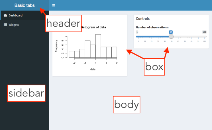
The most basic shinydashboard is made up of a header, a sidebar, and a body
The main difference between a shiny app and a shinydashboard are the UI elements. Rather than a fluidPage() or navbarPage() (as used in our previous shiny apps), we’ll create a dashboardPage(), which expects three main parts: a header, a sidebar, and a body. Below is the most minimal possible UI for a {shinydashboard} page (you can run this code in an app.R file, if you wish).
#..............................setup.............................
library(shiny)
library(shinydashboard)

#...............................ui...............................
ui <- dashboardPage(

  dashboardHeader(),
  dashboardSidebar(),
  dashboardBody()

)

#.............................server.............................
server <- function(input, output) {}

#......................combine ui & server.......................
shinyApp(ui, server)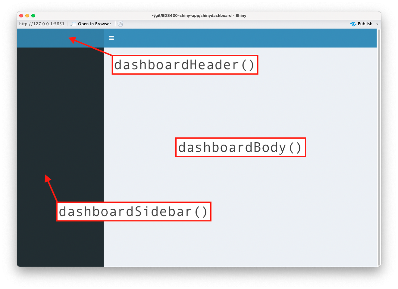
Example shiny dashboards built by some familiar folks
CA Schools Climate Hazards (source code), by MEDS 2024 alumni Charlie Curtin, Kristina Glass, Liane Chen & Hazel Vaquero, as part of their MEDS Capstone project – explore localized climate hazards for 10,000+ public schools in CA. Also runner up in Posit’s 2024 Shiny Contest!!!
Milkweed Site Finder (source code), by MEDS 2024 alumni Amanda Herbst, Anna Ramji, Melissa Widas & Sam Muir, as part of their MEDS Capstone project – a tool for the Santa Barbara Botanic Garden to prioritize Milkweed restoration sites across the Los Padres National Forest
Bren Student Data Explorer (source code), by MEDS 2022 alum, Halina Do-Linh, & MEDS staff – explore Bren school student demographics and career outcomes
Sam’s Strava Stats (source code), by yours truly, Sam Shanny-Csik – a new and ongoing side project exploring my Strava hiking / biking / walking data
Visualizing human impacts on at-risk marine biodiversity (source code), developed by MESM 2022 alum, Ian Brunjes & Dr. Casey O’Hara) – explore how human activities and climate change impact marine biodiversity worldwide
Setup your shiny dashboard
First, create a subdirectory called shinydashboard/ and add a ui.R, server.R, and global.R file.
Add the server function to server.R and the three main UI components (header, sidebar, and body) to our dashboard page – to keep things organized, I recommend splitting the UI into separate pieces, then combining them into a dashboardPage at the end of ui.R
We’ll set our dashboard aside for now while we work on downloading and pre-processing our data, as well as practice creating our data visualization outside of our app.
~/shinydashboard/ui.R
#........................dashboardHeader.........................
header <- dashboardHeader()

#........................dashboardSidebar........................
sidebar <- dashboardSidebar()

#..........................dashboardBody.........................
body <- dashboardBody()

#..................combine all in dashboardPage..................
dashboardPage(header, sidebar, body)Be sure to run your app after each new addition!
From here on out, you should be running your app after each new addition to check that things work as expected – aim to do so after each slide where code is added.
I don’t explicitly call to do so on each slide, but this is a super important practice to get into!
Remember to give yourself proper space between lines and add annotations at the start and end of each parentheses – I highly recommend following along with the formatting I use throughout these materials.
As always, let’s start with the data
Building an app doesn’t make much sense if we don’t know what we’re going to put in it. So, just like the last two apps, we’ll start with some data wrangling and practice data visualization.
Unlike our last two apps, however, we’ll be working with tabular data from the Arctic Data Center, which we’ll download, process, save, then finally, read into our application. This process will likely be more similar to what you’ll encounter when working on your own applications moving forward. Take a few minutes to review the metadata record for the following data set, and download FCWO_lakemonitoringdata_2011_2022_daily.csv:
Christopher Arp, Matthew Whitman, Katie Drew, and Allen Bondurant. 2022. Water depth, surface elevation, and water temperature of lakes in the Fish Creek Watershed in northern Alaska, USA, 2011-2022. Arctic Data Center. doi:10.18739/A2JH3D41P.
![]()
Pre-processing data is critical
Where you choose to store the data used by your Shiny app will depend largely on the type and size of the file(s) and who “owns” those data.
It is likely that you’ll be working with data stored in a database or on a server. This is outside the scope of this workshop, but I suggest reading Nathan Stephens’ article, Where to store your Shiny application data to start. Because we are going to be working with a relatively small data set today, we’ll bundle our data file with our dashboard inside our repository.
Regardless of where you choose to store your data, you can help your application more quickly process inputs / outputs by providing it only as much data as needed to run. This means pre-processing your data.
Pre-processing data is critical
FCWO_lakemonitoringdata_2011_2022_daily.csv contains 8 attributes (variables) and 18,994 observations collected from a set of 11 lakes located in the Fish Creek Watershed in northern Alaska between 2011-2022. We’ll:
download and save the file to a raw-data/ folder in the root directory of our repository
pre-process the data in a separate script(s) saved to scratch/
save a cleaned / processed version of the data to our app’s directory, /shinydashboard/data/lake_data_processed.csv.
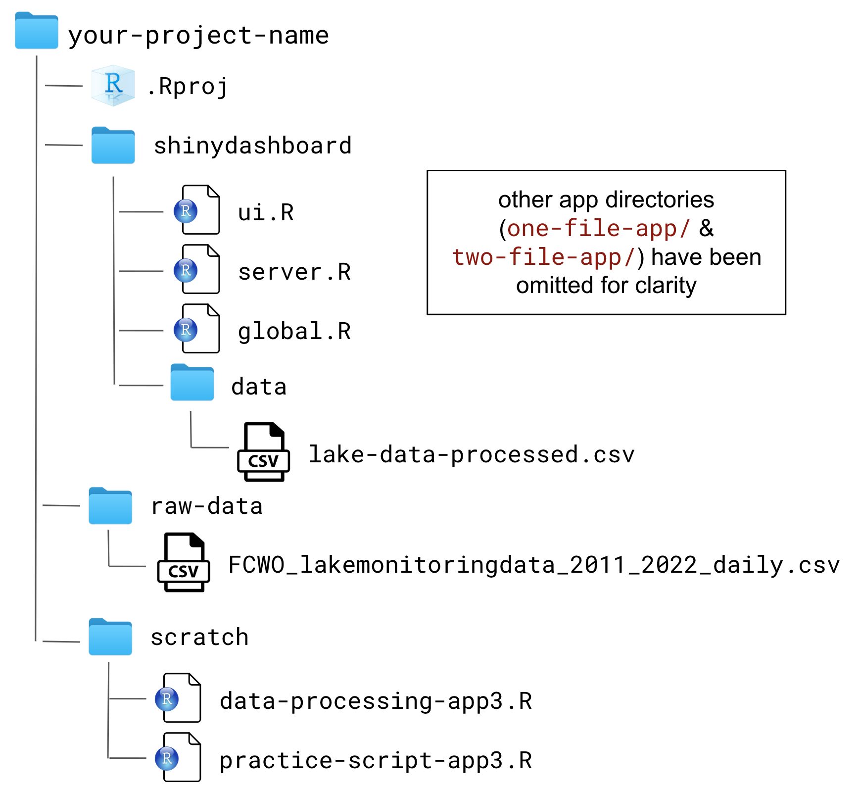
Your repository structure should look similar to example, above.
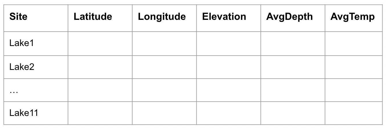
The goal:
Our goal is to create a leaflet map with makers placed on each of the 11 unique lakes where data were collected. When clicked, a marker should reveal the lake name, elevation (in meters, above sea level), average depth of the lake (in meters), and average lake bed temperature (in degrees Celsius). To do so, we’ll need a data frame that looks like the example below:
Process lake data & save new file
~/scratch/data-processing-app3.R
#...............................................................................
#                                                                              .
#  For simplicity, I've removed all rows with missing values (i.e. `NaN`s      .
#  in the `Depth` column & `NA`s in the `BedTemperature` column) before        .
#  calculating averages. However, exploring and  thinking critically about     .
#  missing data is an important part of data analysis, and in a real-life      .
#  scenario, you should consider the most appropriate method for handling them .
#                                                                              .
#...............................................................................

#....................SETUP & DATA PROCESSING.....................

# load packages ----
library(tidyverse)
library(arrow) # see next slide

# read in raw data ----
lake_raw <- read_csv(here::here("raw-data", "FCWO_lakemonitoringdata_2011_2022_daily.csv"))

# calculate avg depth & temp ----
avg_depth_temp <- lake_raw |>
  select(Site, Depth, BedTemperature) |>
  filter(Depth != "NaN") |>  # remove NaN ("not a number") from Depth
  drop_na(BedTemperature) |> # remove NAs (missing data) from BedTemperature
  group_by(Site) |>
  summarize(
    AvgDepth = round(mean(Depth), 1),
    AvgTemp = round(mean(BedTemperature), 1)
    )

# join avg depth & temp to original data (match rows based on 'Site') ---
joined_dfs <- full_join(lake_raw, avg_depth_temp)

# get unique lakes observations (with corresponding lat, lon, elev, avgDepth, avgTemp) for mapping ----
unique_lakes <- joined_dfs |>
  select(Site, Latitude, Longitude, Elevation, AvgDepth, AvgTemp) |>
  distinct()

# save processed data to your app's data directory (here, we're saving as both .csv and .parquet) ----
write_csv(x = unique_lakes, file = here::here("shinydashboard", "data", "lake_data_processed.csv"))
arrow::write_parquet(x = unique_lakes, sink = here::here("shinydashboard", "data", "lake_data_processed.parquet"))
A note on file types
You may choose to save your processed data frame as a .parquet file (a columnar data format designed for efficient storage and retrieval). .parquet files are small due to built-in compression, fast to import/export, and preserve data types and classes (e.g. factors and dates), eliminating the need to redefine data types after loading. Unlike .rds files, which are native to R only, .parquet files are language-agnostic, which means you can read them in R, Python, and many other tools. This makes them a great choice if you’re working across languages or sharing data with others.
For buiding apps, we recommend .parquet over .csv because CSV files don’t preserve data types (meaning you’ll need to redefine factors, dates, etc. after every import) and are slower to read/write at scale. You can read in and write out .parquet files using the {arrow} package (arrow::read_parquet() / arrow::write_parquet()) just as easily as .csv files.


Note: If you’re sharing data with someone who needs to open it directly (e.g. in Excel), .csv is the better choice due to it’s plain text format, which is readable by any standard software. .parquet is a binary format that requires specialized tools to view, so it’s best suited for data you’ll be reading programmatically.
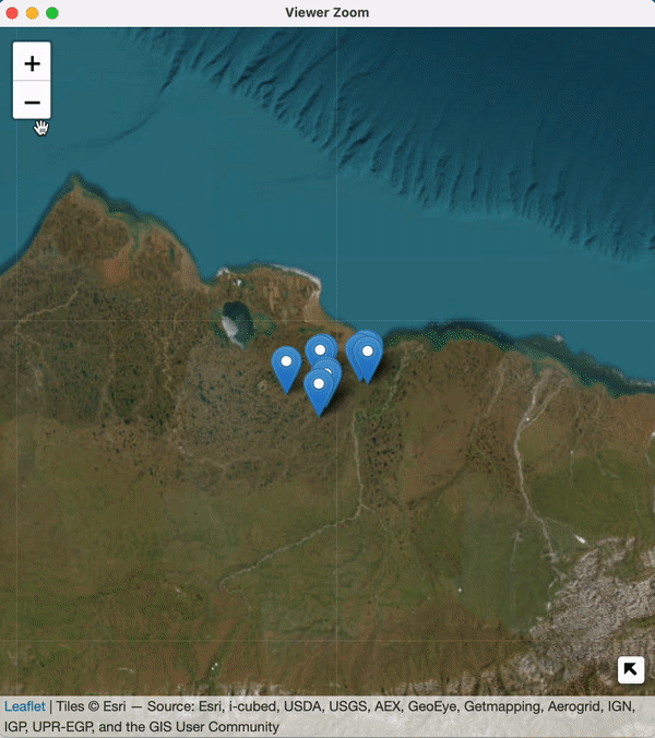
Draft leaflet map
There are lots of ways to customize leaflet maps. We’ll be keeping ours relatively simple, but check out the Leaflet for R documentation for more ways to get creative with your maps.
~/scratch/practice-script-app3.R
#..............................SETUP.............................

# load packages ----
library(arrow)
library(leaflet)

# read in data ----
lake_data <- read_parquet(here::here("shinydashboard", "data", "lake_data_processed.parquet"))

#..........................PRACTICE VIZ..........................
leaflet() |>

  # add tiles
  addProviderTiles(providers$Esri.WorldImagery) |>

  # set view over AK
  setView(lng = -152.048442, lat = 70.249234, zoom = 6) |>

  # add mini map
  addMiniMap(toggleDisplay = TRUE, minimized = FALSE) |>

  # add markers
  addMarkers(data = lake_data,
             lng = lake_data$Longitude, lat = lake_data$Latitude,
             popup = paste0("Site Name: ", lake_data$Site, "<br>",
                           "Elevation: ", lake_data$Elevation, " meters (above SL)", "<br>",
                           "Avg Depth: ", lake_data$AvgDepth, " meters", "<br>",
                           "Avg Lake Bed Temperature: ", lake_data$AvgTemp, "°C")) # NOTE: Shift + Option + 8 (mac), Alt + 0176 (Windows), or use unicode "\u00B0C"
Practice filtering leaflet observations
We’ll eventually build three sliderInputs to filter lake makers by Elevation, AvgDepth, and AvgTemp. Practice filtering here first (and be sure to update the data frame name in your leaflet code!):
~/scratch/practice-script-app3.R
#..............................SETUP.............................

# load packages ----
library(arrow)
library(tidyverse)
library(leaflet)

# read in data ----
lake_data <- read_parquet(here::here("shinydashboard", "data", "lake_data_processed.parquet"))

#.......................PRACTICE FILTERING.......................

filtered_lakes_df <- lake_data |>
  filter(Elevation >= 8 & Elevation <= 20) |>
  filter(AvgDepth >= 2 & AvgDepth <= 3) |>
  filter(AvgTemp >= 4 & AvgTemp <= 6)

#..........................PRACTICE VIZ..........................

leaflet() |>

  # add tiles
  addProviderTiles(providers$Esri.WorldImagery, # make note of using appropriate tiles
                   options = providerTileOptions(maxNativeZoom = 19, maxZoom = 100)) |>

  # add mini map
  addMiniMap(toggleDisplay = TRUE, minimized = TRUE) |>

  # set view over AK
  setView(lng = -152.048442, lat = 70.249234, zoom = 6) |>

  # add markers
  addMarkers(data = filtered_lakes_df,
             lng = filtered_lakes_df$Longitude, lat = filtered_lakes_df$Latitude,
             popup = paste0("Site Name: ", filtered_lakes_df$Site, "<br>",
                           "Elevation: ", filtered_lakes_df$Elevation, " meters (above SL)", "<br>",
                           "Avg Depth: ", filtered_lakes_df$AvgDepth, " meters", "<br>",
                           "Avg Lake Bed Temperature: ", filtered_lakes_df$AvgTemp, "°C")) # NOTE: Shift + Option + 8 (mac), Alt + 0176 (Windows), or use unicode "\u00B0C"
Sketch out our dashboard UI
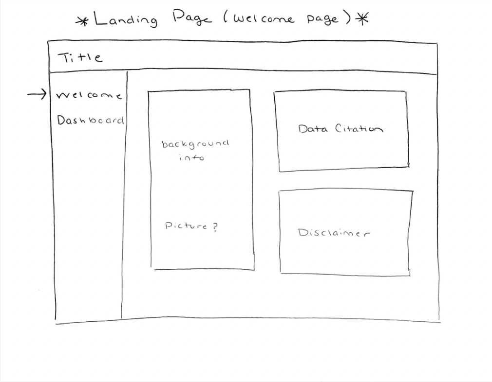
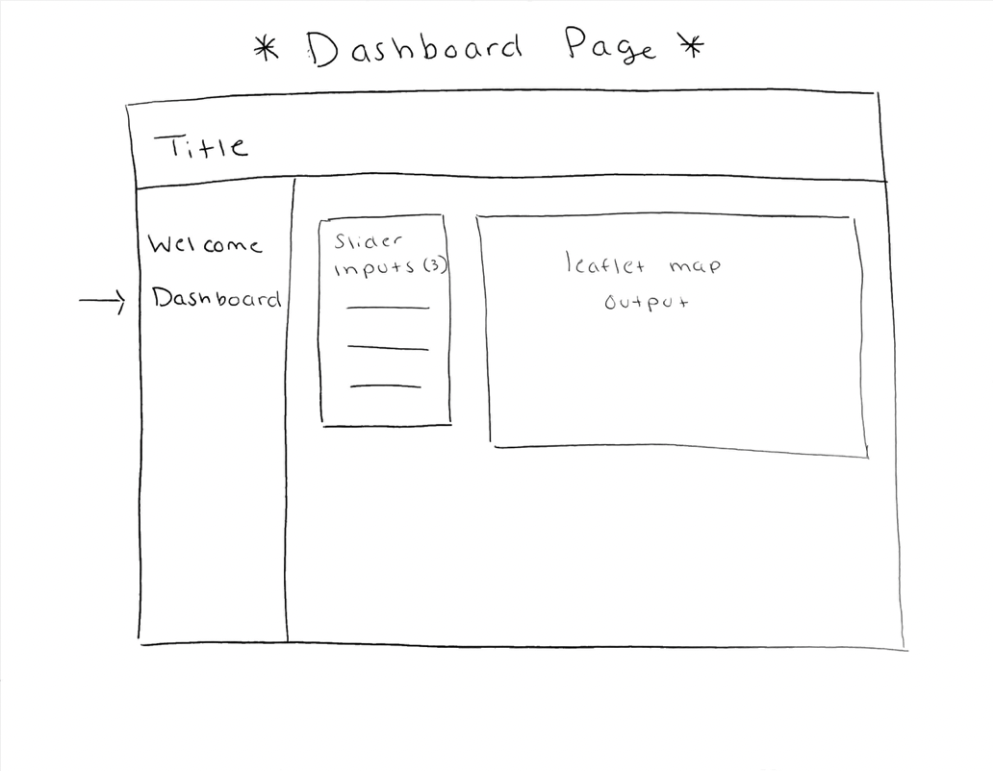
I want my dashboard to have two menu items: a welcome page with some background information, and a dashboard page with my reactive map. All elements will be placed inside boxes, the primary building blocks of shinydashboards (more on that soon).
Add a title & menuItems
First, add a title to dashboardHeader() and make more space using titleWidth, if necessary.
Next, we’ll build our dashboardSidebar(). Add a sidebarMenu() that contains two menuItems. Be sure to provide each menuItem() with text as you’d like it to appear in your app (for me, that’s Welcome and Dashboard), and a tabName which will be used to place dashboardBody() content in the appropriate menuItem(). Optionally, you can provide an icon. By default, icon() uses icons from FontAwesome.
~/shinydashboard/ui.R
#........................dashboardHeader.........................
header <- dashboardHeader(

  # title ----
  title = "Fish Creek Watershed Lake Monitoring",
  titleWidth = 400

) # END dashboardHeader

#........................dashboardSidebar........................
sidebar <- dashboardSidebar(

  # sidebarMenu ----
  sidebarMenu(

    menuItem(text = "Welcome", tabName = "welcome", icon = icon("star")),
    menuItem(text = "Dashboard", tabName = "dashboard", icon = icon("gauge"))

  ) # END sidebarMenu

) # END dashboardSidebar

#..........................dashboardBody.........................
body <- dashboardBody()

#..................combine all in dashboardPage..................
dashboardPage(header, sidebar, body)
Add tabItems to your dashboardBody
Next, we’ll create tabItems in our dashboardBody – we’ll make a tabItem (singular) for each menuItem in our dashboardSidebar. In order to match a menuItem and a tabItem, ensure that they have matching a tabName (e.g. any content added to the dashboard tabItem will appear under the dashboard menuItem).
~/shinydashboard/ui.R
#........................dashboardHeader.........................
header <- dashboardHeader(

  # add title ----
  title = "Fish Creek Watershed Lake Monitoring",
  titleWidth = 400

) # END dashboardHeader

#........................dashboardSidebar........................
sidebar <- dashboardSidebar(

  # sidebarMenu ----
  sidebarMenu(

    menuItem(text = "Welcome", tabName = "welcome", icon = icon("star")),
    menuItem(text = "Dashboard", tabName = "dashboard", icon = icon("gauge"))

  ) # END sidebarMenu

) # END dashboardSidebar

#..........................dashboardBody.........................
body <- dashboardBody(

  # tabItems ----
  tabItems(

    # welcome tabItem ----
    tabItem(tabName = "welcome",

            "background info here"

    ), # END welcome tabItem

    # dashboard tabItem ----
    tabItem(tabName = "dashboard",

            "dashboard content here"

    ) # END dashboard tabItem

  ) # END tabItems

) # END dashboardBody

#..................combine all in dashboardPage..................
dashboardPage(header, sidebar, body)
Add boxes to contain UI content (part 1)
Boxes are the primary building blocks of shinydashboards and can contain almost any Shiny UI element (e.g. text, inputs, outputs). Start by adding two side-by-side boxes to our dashboard tab. Together, their widths will add up to 12 (the total width of a browser page). These boxes will eventually contain our sliderInputs and our leafletOutput.
~/shinydashboard/ui.R
#........................dashboardHeader.........................
header <- dashboardHeader(

  # add title ----
  title = "Fish Creek Watershed Lake Monitoring",
  titleWidth = 400

) # END dashboardHeader

#........................dashboardSidebar........................
sidebar <- dashboardSidebar(

  # sidebarMenu ----
  sidebarMenu(

    menuItem(text = "Welcome", tabName = "welcome", icon = icon("star")),
    menuItem(text = "Dashboard", tabName = "dashboard", icon = icon("gauge"))

  ) # END sidebarMenu

) # END dashboardSidebar

#..........................dashboardBody.........................
body <- dashboardBody(

  # tabItems ----
  tabItems(

    # welcome tabItem ----
    tabItem(tabName = "welcome",

            "background info here"

    ), # END welcome tabItem

    # dashboard tabItem ----
    tabItem(tabName = "dashboard",

            # input box ----
            box(width = 4,

                "sliderInputs here"

            ), # END input box

            # leaflet box ----
            box(width = 8,

                "leafletOutput here"

            ) # END leaflet box

    ) # END dashboard tabItem

  ) # END tabItems

) # END dashboardBody

#..................combine all in dashboardPage..................
dashboardPage(header, sidebar, body)
Add boxes to contain UI content (part 2)
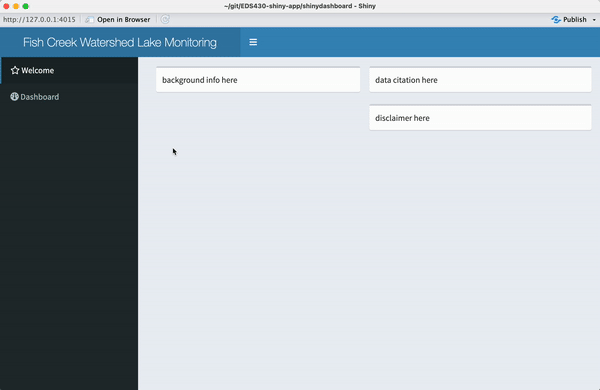
Lastly, add boxes to our welcome tab We’ll use columns to place one box on the left-hand side of our page, and two stacked boxes on the right-hand side. Each column will take up half the page (Note: For column-based layouts, use NULL for the box width, as the width is set by the column that contains the box).
~/shinydashboard/ui.R
#........................dashboardHeader.........................
header <- dashboardHeader(

  # add title ----
  title = "Fish Creek Watershed Lake Monitoring",
  titleWidth = 400

) # END dashboardHeader

#........................dashboardSidebar........................
sidebar <- dashboardSidebar(

  # sidebarMenu ----
  sidebarMenu(

    menuItem(text = "Welcome", tabName = "welcome", icon = icon("star")),
    menuItem(text = "Dashboard", tabName = "dashboard", icon = icon("gauge"))

  ) # END sidebarMenu

) # END dashboardSidebar

#..........................dashboardBody.........................
body <- dashboardBody(

  # tabItems ----
  tabItems(

    # welcome tabItem ----
    tabItem(

      tabName = "welcome",

      # left-hand column ----
      column(width = 6,

        # background info box ----
        box(width = NULL,

          "background info here"

        ) # END background info box

      ), # END left-hand column

      # right-hand column ----
      column(width = 6,

        # data source box ----
        box(width = NULL,

          "data citation here"

        ), # END data source box

        # disclaimer box ----
        box(width = NULL,

          "disclaimer here"

        ) # END disclaimer box

      ) # END right-hand column

    ), # END welcome tabItem

    # dashboard tabItem ----
    tabItem(

      tabName = "dashboard",

      # input box ----
      box(width = 4,

        "sliderInputs here"

      ), # END input box

      # leaflet box ----
      box(width = 8,

        "leafletOutput here"

      ) # END leaflet box

    ) # END dashboard tabItem

  ) # END tabItems

) # END dashboardBody

#..................combine all in dashboardPage..................
dashboardPage(header, sidebar, body)
Read data into global.R & add necessary packages
Remember to load your pre-processed data, which should live in the data/ folder within your app’s directory.
Some important notes:
here::here() in your shiny apps, since Shiny sets the working directory to the app’s directory automatically. Using {here} can cause some unexpected issues (read more about it in this discussion)ui.R, server.R). It’s important to note, however, that you won’t be able to run your code line-by-line (like in a typical script; the file path won’t be recognized) – this is expected!.Add a sliderInput & leafletOutput to the UI
Start by adding just one sliderInput (for selecting a range of lake Elevations) to the left-hand box in the dashboard tab. Then, add a leafletOutput to create a placeholder space for our map, along with a Spinner animation (from the {shinycssloaders} package). While we’re here, we can also add titles to each box.
~/shinydashboard/ui.R
#........................dashboardHeader.........................
header <- dashboardHeader(

  # add title ----
  title = "Fish Creek Watershed Lake Monitoring",
  titleWidth = 400

) # END dashboardHeader

#........................dashboardSidebar........................
sidebar <- dashboardSidebar(

  # sidebarMenu ----
  sidebarMenu(

    menuItem(text = "Welcome", tabName = "welcome", icon = icon("star")),
    menuItem(text = "Dashboard", tabName = "dashboard", icon = icon("gauge"))

  ) # END sidebarMenu

) # END dashboardSidebar

#..........................dashboardBody.........................
body <- dashboardBody(

  # tabItems ----
  tabItems(

    # welcome tabItem ----
    tabItem(tabName = "welcome",

      # left-hand column ----
      column(width = 6,

        # background info box ----
        box(width = NULL,

          "background info here"

        ) # END background info box

      ), # END left-hand column

      # right-hand column ----
      column(width = 6,

        # data source box ----
        box(width = NULL,

          "data citation here"

        ), # END data source box

        # disclaimer box ----
        box(width = NULL,

          "disclaimer here"

        ) # END disclaimer box

      ) # END right-hand column

    ), # END welcome tabItem

    # dashboard tabItem ----
    tabItem(tabName = "dashboard",

      # input box ----
      box(width = 4,

        title = tags$strong("Adjust lake parameter ranges:"),

        # sliderInputs ----
        sliderInput(inputId = "elevation_slider_input",
                    label = "Elevation (meters above SL):",
                    min = min(lake_data$Elevation),
                    max = max(lake_data$Elevation),
                    value = c(min(lake_data$Elevation), max(lake_data$Elevation)))

      ), # END input box

      # leaflet box ----
      box(width = 8,

        title = tags$strong("Monitored lakes within Fish Creek Watershed:"),

        # leafletOutput ----
        leafletOutput(outputId = "lake_map_output") |>
          withSpinner(type = 1, color = "#4287f5")

      ) # END leaflet box

    ) # END dashboard tabItem

  ) # END tabItems

) # END dashboardBody

#..................combine all in dashboardPage..................
dashboardPage(header, sidebar, body)
Assemble inputs & outputs in server.R
Remember to reference your practice data viz script and to follow our three steps for creating reactive outputs. And don’t forget to add () following each reactive data frame called in your leaflet map!
~/shinydashboard/server.R
server <- function(input, output) {

  ##~~~~~~~~~~~~~~~~~~~~~~~~~~~~~~~~~~~~~~~~~~~~~~~~~~~~~~~~~~~~~~~~~~~~~~~~~~~~~~
  ##                                leaflet map                               ----
  ##~~~~~~~~~~~~~~~~~~~~~~~~~~~~~~~~~~~~~~~~~~~~~~~~~~~~~~~~~~~~~~~~~~~~~~~~~~~~~~

  #........................filter lake data........................
  filtered_lakes_df <- reactive ({

    lake_data |>
      filter(Elevation >= input$elevation_slider_input[1] & Elevation <= input$elevation_slider_input[2])

  })

  #........................build leaflet map.......................
  output$lake_map_output <- renderLeaflet({

    leaflet() |>

      # add tiles
      addProviderTiles(providers$Esri.WorldImagery) |>

      # set view over AK
      setView(lng = -152.048442, lat = 70.249234, zoom = 6) |>

      # add mini map
      addMiniMap(toggleDisplay = TRUE, minimized = TRUE) |>

      # add markers
      addMarkers(data =  filtered_lakes_df(),
                 lng = filtered_lakes_df()$Longitude,
                 lat = filtered_lakes_df()$Latitude,
                 popup = paste("Site Name:", filtered_lakes_df()$Site, "<br>",
                               "Elevation:", filtered_lakes_df()$Elevation, "meters (above SL)", "<br>",
                               "Avg Depth:", filtered_lakes_df()$AvgDepth, "meters", "<br>",
                               "Avg Lake Bed Temperature:", filtered_lakes_df()$AvgTemp, "°C"))

  })

}
Run your app & test out your first widget
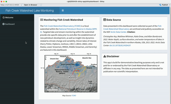
If all is good, you should see something similar to this:
Exercise 5: Add two more sliderInputs to filter for AvgDepth & AvgTemp
To Do:
Add two more sliderInputs, one for AvgDepth and one for AvgTemp beneath our first Elevation sliderInput in the UI
Update our reactive data frame so that all three widgets filter the leaflet map
See next slide for a solution!
Exercise 5: A solution
~/shinydashboard/ui.R
#........................dashboardHeader.........................
header <- dashboardHeader(

  # add title ----
  title = "Fish Creek Watershed Lake Monitoring",
  titleWidth = 400

) # END dashboardHeader

#........................dashboardSidebar........................
sidebar <- dashboardSidebar(

  # sidebarMenu ----
  sidebarMenu(

    menuItem(text = "Welcome", tabName = "welcome", icon = icon("star")),
    menuItem(text = "Dashboard", tabName = "dashboard", icon = icon("gauge"))

  ) # END sidebarMenu

) # END dashboardSidebar

#..........................dashboardBody.........................
body <- dashboardBody(

  # tabItems ----
  tabItems(

    # welcome tabItem ----
    tabItem(tabName = "welcome",

      # left-hand column ----
      column(width = 6,

        # background info box ----
        box(width = NULL,

          "background info here"

        ) # END background info box

      ), # END left-hand column

      # right-hand column ----
      column(width = 6,

        # data source box ----
        box(width = NULL,

          "data citation here"

        ), # END data source box

        # disclaimer box ----
        box(width = NULL,

          "disclaimer here"

        ) # END disclaimer box

      ) # END right-hand column

    ), # END welcome tabItem

    # dashboard tabItem ----
    tabItem(tabName = "dashboard",

      # input box ----
      box(width = 4,

        title = tags$strong("Adjust lake parameter ranges:"),

        # sliderInputs ----
        sliderInput(inputId = "elevation_slider_input",
                    label = "Elevation (meters above SL):",
                    min = min(lake_data$Elevation),
                    max = max(lake_data$Elevation),
                    value = c(min(lake_data$Elevation), max(lake_data$Elevation))),

        sliderInput(inputId = "depth_slider_input",
                    label = "Average depth (meters):",
                    min = min(lake_data$AvgDepth),
                    max = max(lake_data$AvgDepth),
                    value = c(min(lake_data$AvgDepth), max(lake_data$AvgDepth))),

        sliderInput(inputId = "temp_slider_input",
                    label = "Average lake bed temperature (°C):",
                    min = min(lake_data$AvgTemp),
                    max = max(lake_data$AvgTemp),
                    value = c(min(lake_data$AvgTemp), max(lake_data$AvgTemp)))

      ), # END input box

      # leaflet box ----
      box(width = 8,

        title = tags$strong("Monitored lakes within Fish Creek Watershed:"),

        # leafletOutput ----
        leafletOutput(outputId = "lake_map_output") |>
          withSpinner(type = 1, color = "#4287f5")

      ) # END leaflet box

    ) # END dashboard tabItem

  ) # END tabItems

) # END dashboardBody

#..................combine all in dashboardPage..................
dashboardPage(header, sidebar, body)
~/shinydashboard/server.R
server <- function(input, output) {

  ##~~~~~~~~~~~~~~~~~~~~~~~~~~~~~~~~~~~~~~~~~~~~~~~~~~~~~~~~~~~~~~~~~~~~~~~~~~~~~~
  ##                                leaflet map                               ----
  ##~~~~~~~~~~~~~~~~~~~~~~~~~~~~~~~~~~~~~~~~~~~~~~~~~~~~~~~~~~~~~~~~~~~~~~~~~~~~~~

  #........................filter lake data........................
  filtered_lakes_df <- reactive ({

    lake_data |>
      filter(Elevation >= input$elevation_slider_input[1] & Elevation <= input$elevation_slider_input[2])  |>
      filter(AvgDepth >= input$depth_slider_input[1] & AvgDepth <= input$depth_slider_input[2]) |>
      filter(AvgTemp >= input$temp_slider_input[1] & AvgTemp <= input$temp_slider_input[2])

  })

  #........................build leaflet map.......................
  output$lake_map_output <- renderLeaflet({

    leaflet() |>

      # add tiles
      addProviderTiles(providers$Esri.WorldImagery) |>

      # set view over AK
      setView(lng = -152.048442, lat = 70.249234, zoom = 6) |>

      # add mini map
      addMiniMap(toggleDisplay = TRUE, minimized = TRUE) |>

      # add markers
      addMarkers(data =  filtered_lakes_df(),
                 lng = filtered_lakes_df()$Longitude,
                 lat = filtered_lakes_df()$Latitude,
                 popup = paste("Site Name:", filtered_lakes_df()$Site, "<br>",
                               "Elevation:", filtered_lakes_df()$Elevation, "meters (above SL)", "<br>",
                               "Avg Depth:", filtered_lakes_df()$AvgDepth, "meters", "<br>",
                               "Avg Lake Bed Temperature:", filtered_lakes_df()$AvgTemp, "°C"))

  })

}
& Exercise 6: Add titles & text to Welcome page boxes
To Do:
text/ folder within your app’s directory and add three markdown (.md) files. Write / format text for the background info (left), data citation (top-right), and disclaimer (bottom-right) boxes. Example text below:~/shinydashboard/text/intro.md
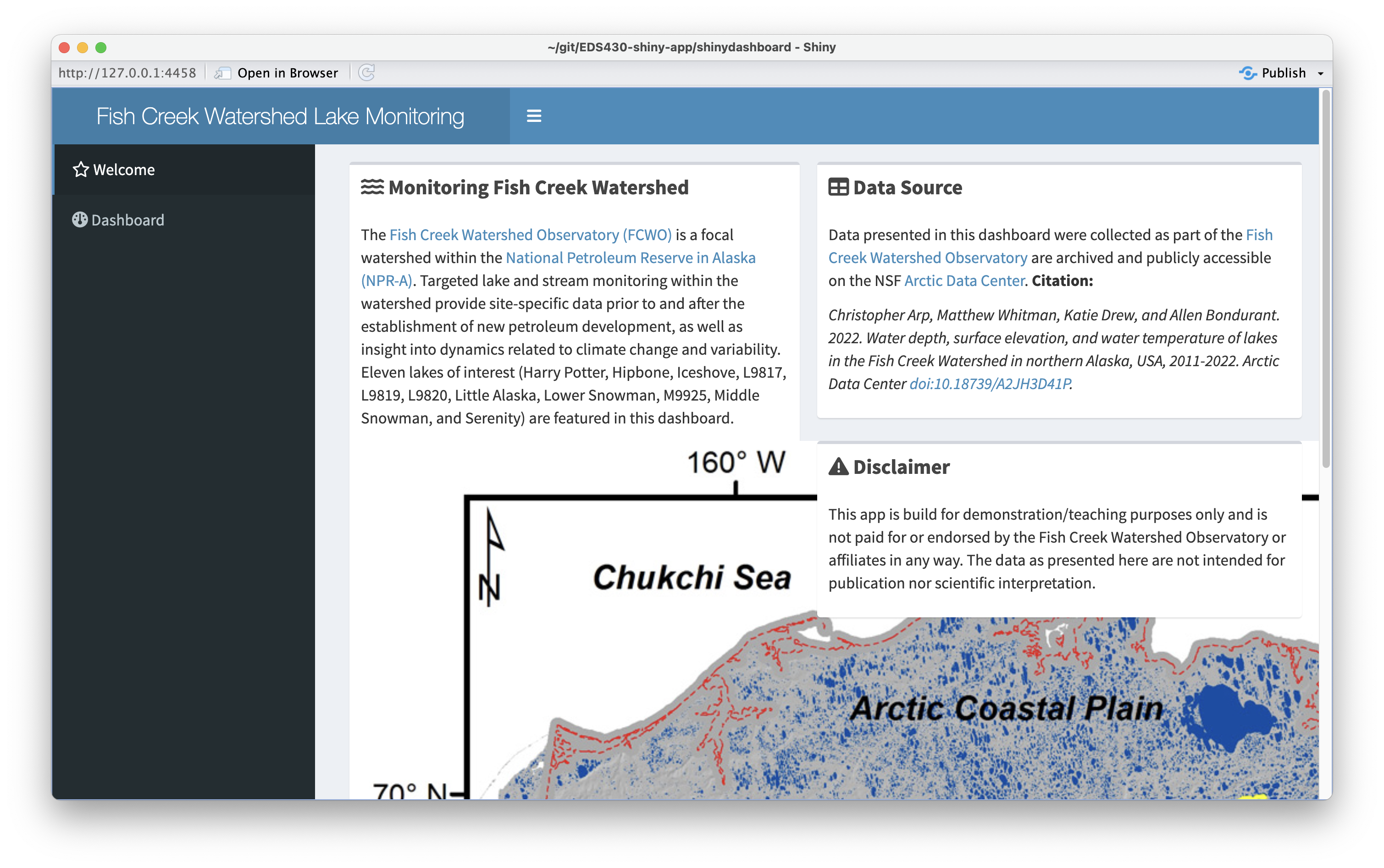
The [Fish Creek Watershed Observatory (FCWO)](http://www.fishcreekwatershed.org/) is a focal watershed within the [National Petroleum Reserve in Alaska (NPR-A)](https://www.blm.gov/programs/energy-and-minerals/oil-and-gas/about/alaska/NPR-A). Targeted lake and stream monitoring within the watershed provide site-specific data prior to and after the establishment of new petroleum development, as well as insight into dynamics related to climate change and variability. Eleven lakes of interest (Harry Potter, Hipbone, Iceshove, L9817, L9819, L9820, Little Alaska, Lower Snowman, M9925, Middle Snowman, and Serenity) are featured in this dashboard.~/shinydashboard/text/citation.md
Data presented in this dashboard were collected as part of the [Fish Creek Watershed Observatory](http://www.fishcreekwatershed.org/) are archived and publicly accessible on the NSF [Arctic Data Center](https://arcticdata.io/). **Citation:**

*Christopher Arp, Matthew Whitman, Katie Drew, and Allen Bondurant. 2022. Water depth, surface elevation, and water temperature of lakes in the Fish Creek Watershed in northern Alaska, USA, 2011-2022. Arctic Data Center [doi:10.18739/A2JH3D41P](https://arcticdata.io/catalog/view/doi%3A10.18739%2FA2JH3D41P).*Tips:
title = tagList(icon("icon-name"), strong("title text here"))Exercise 6: A solution
Press the right arrow key to advance through the newly added lines of code.
~/shinydashboard/ui.R
#........................dashboardHeader.........................
header <- dashboardHeader(

  # add title ----
  title = "Fish Creek Watershed Lake Monitoring",
  titleWidth = 400

) # END dashboardHeader

#........................dashboardSidebar........................
sidebar <- dashboardSidebar(

  # sidebarMenu ----
  sidebarMenu(

    menuItem(text = "Welcome", tabName = "welcome", icon = icon("star")),
    menuItem(text = "Dashboard", tabName = "dashboard", icon = icon("gauge"))

  ) # END sidebarMenu

) # END dashboardSidebar

#..........................dashboardBody.........................
body <- dashboardBody(

  # tabItems ----
  tabItems(

    # welcome tabItem ----
    tabItem(tabName = "welcome",

            # left-hand column ----
            column(width = 6,

                   # background info box ----
                   box(width = NULL,

                       title = tagList(icon("water"), strong("Monitoring Fish Creek Watershed")),
                       includeMarkdown("text/intro.md")

                   ) # END background info box

            ), # END left-hand column

            # right-hand column ----
            column(width = 6,

                   # data source box ----
                   box(width = NULL,

                       title = tagList(icon("table"), strong("Data Source")),
                       includeMarkdown("text/citation.md")

                   ), # END data source box

                   # disclaimer box ----
                   box(width = NULL,

                       title = tagList(icon("triangle-exclamation"), strong("Disclaimer")),
                       includeMarkdown("text/disclaimer.md")

                   ) # END disclaimer box

            ) # END right-hand column

    ), # END welcome tabItem

    # dashboard tabItem ----
    tabItem(tabName = "dashboard",

            # input box ----
            box(width = 4,

                title = tags$strong("Adjust lake parameter ranges:"),

                # sliderInputs ----
                sliderInput(inputId = "elevation_slider_input",
                            label = "Elevation (meters above SL):",
                            min = min(lake_data$Elevation),
                            max = max(lake_data$Elevation),
                            value = c(min(lake_data$Elevation), max(lake_data$Elevation))),

                sliderInput(inputId = "depth_slider_input",
                            label = "Average depth (meters):",
                            min = min(lake_data$AvgDepth),
                            max = max(lake_data$AvgDepth),
                            value = c(min(lake_data$AvgDepth), max(lake_data$AvgDepth))),

                sliderInput(inputId = "temp_slider_input",
                            label = "Average lake bed temperature (°C):",
                            min = min(lake_data$AvgTemp),
                            max = max(lake_data$AvgTemp),
                            value = c(min(lake_data$AvgTemp), max(lake_data$AvgTemp)))

            ), # END input box

            # leaflet box ----
            box(width = 8,

                title = tags$strong("Monitored lakes within Fish Creek Watershed:"),

                # leafletOutput ----
                leafletOutput(outputId = "lake_map_output") |>
                  withSpinner(type = 1, color = "#4287f5")

            ) # END leaflet box

    ) # END dashboard tabItem

  ) # END tabItems

) # END dashboardBody

#..................combine all in dashboardPage..................
dashboardPage(header, sidebar, body)
Add a static image
Let’s add an image to the Welcome page, inside the left-hand box beneath our intro text. First, create a www/ folder inside your app’s directory (refer back to part 1.2. Download the map of the Fish Creek Watershed from FCWO’s website and save it to your www/ directory.
Next, use the img tag to add your image. Supply a file path, relative to your www/ directory, using the src argument, and add alt text using the alt argument.
~/shinydashboard/ui.R
#........................dashboardHeader.........................
header <- dashboardHeader(

  # add title ----
  title = "Fish Creek Watershed Lake Monitoring",
  titleWidth = 400

) # END dashboardHeader

#........................dashboardSidebar........................
sidebar <- dashboardSidebar(

  # sidebarMenu ----
  sidebarMenu(

    menuItem(text = "Welcome", tabName = "welcome", icon = icon("star")),
    menuItem(text = "Dashboard", tabName = "dashboard", icon = icon("gauge"))

  ) # END sidebarMenu

) # END dashboardSidebar

#..........................dashboardBody.........................
body <- dashboardBody(

  # tabItems ----
  tabItems(

    # welcome tabItem ----
    tabItem(tabName = "welcome",

            # left-hand column ----
            column(width = 6,

                   # background info box ----
                   box(width = NULL,

                       title = tagList(icon("water"), strong("Monitoring Fish Creek Watershed")),
                       includeMarkdown("text/intro.md"),
                       tags$img(src = "FishCreekWatershedSiteMap_2020.jpg",
                                alt = "A map of northern Alaska, showing Fish Creek Watershed located within the National Petroleum Reserve.")

                   ) # END background info box

            ), # END left-hand column

            # right-hand column ----
            column(width = 6,

                   # data source box ----
                   box(width = NULL,

                       title = tagList(icon("table"), strong("Data Source")),
                       includeMarkdown("text/citation.md")

                   ), # END data source box

                   # disclaimer box ----
                   box(width = NULL,

                       title = tagList(icon("triangle-exclamation"), strong("Disclaimer")),
                       includeMarkdown("text/disclaimer.md")

                   ) # END disclaimer box

            ) # END right-hand column

    ), # END welcome tabItem

    # dashboard tabItem ----
    tabItem(tabName = "dashboard",

            # input box ----
            box(width = 4,

                title = tags$strong("Adjust lake parameter ranges:"),

                # sliderInputs ----
                sliderInput(inputId = "elevation_slider_input",
                            label = "Elevation (meters above SL):",
                            min = min(lake_data$Elevation),
                            max = max(lake_data$Elevation),
                            value = c(min(lake_data$Elevation), max(lake_data$Elevation))),

                sliderInput(inputId = "depth_slider_input",
                            label = "Average depth (meters):",
                            min = min(lake_data$AvgDepth),
                            max = max(lake_data$AvgDepth),
                            value = c(min(lake_data$AvgDepth), max(lake_data$AvgDepth))),

                sliderInput(inputId = "temp_slider_input",
                            label = "Average lake bed temperature (°C):",
                            min = min(lake_data$AvgTemp),
                            max = max(lake_data$AvgTemp),
                            value = c(min(lake_data$AvgTemp), max(lake_data$AvgTemp)))

            ), # END input box

            # leaflet box ----
            box(width = 8,

                title = tags$strong("Monitored lakes within Fish Creek Watershed:"),

                # leafletOutput ----
                leafletOutput(outputId = "lake_map_output") |>
                  withSpinner(type = 1, color = "#4287f5")

            ) # END leaflet box

    ) # END dashboard tabItem

  ) # END tabItems

) # END dashboardBody

#..................combine all in dashboardPage..................
dashboardPage(header, sidebar, body)
Our image doesn’t look so great as-is…
Use in-line CSS to adjust the image size
We can use in-line CSS to style our image element. It’s okay if you don’t fully understand what’s going on here for now – we’ll talk in greater detail about how CSS (and Sass) can be used to customize the appearance of your apps in just a bit.
Let’s also add a caption below our image that links to the image source, and use in-line CSS to center that text within the box.
~/shinydashboard/ui.R
#........................dashboardHeader.........................
header <- dashboardHeader(

  # add title ----
  title = "Fish Creek Watershed Lake Monitoring",
  titleWidth = 400

) # END dashboardHeader

#........................dashboardSidebar........................
sidebar <- dashboardSidebar(

  # sidebarMenu ----
  sidebarMenu(

    menuItem(text = "Welcome", tabName = "welcome", icon = icon("star")),
    menuItem(text = "Dashboard", tabName = "dashboard", icon = icon("gauge"))

  ) # END sidebarMenu

) # END dashboardSidebar

#..........................dashboardBody.........................
body <- dashboardBody(

  # tabItems ----
  tabItems(

    # welcome tabItem ----
    tabItem(tabName = "welcome",

            # left-hand column ----
            column(width = 6,

                   # background info box ----
                   box(width = NULL,

                       title = tagList(icon("water"), strong("Monitoring Fish Creek Watershed")),
                       includeMarkdown("text/intro.md"),
                       tags$img(src = "FishCreekWatershedSiteMap_2020.jpg",
                                alt = "A map of northern Alaska, showing Fish Creek Watershed located within the National Petroleum Reserve.",
                                style = "max-width: 100%"),
                       tags$p(tags$em("Map Source: ", tags$a(href = "http://www.fishcreekwatershed.org/", "FCWO")),
                              style = "text-align: center;")

                   ) # END background info box

            ), # END left-hand column

            # right-hand column ----
            column(width = 6,

                   # data source box ----
                   box(width = NULL,

                       title = tagList(icon("table"), strong("Data Source")),
                       includeMarkdown("text/citation.md")

                   ), # END data source box

                   # disclaimer box ----
                   box(width = NULL,

                       title = tagList(icon("triangle-exclamation"), strong("Disclaimer")),
                       includeMarkdown("text/disclaimer.md")

                   ) # END disclaimer box

            ) # END right-hand column

    ), # END welcome tabItem

    # dashboard tabItem ----
    tabItem(tabName = "dashboard",

            # input box ----
            box(width = 4,

                title = tags$strong("Adjust lake parameter ranges:"),

                # sliderInputs ----
                sliderInput(inputId = "elevation_slider_input",
                            label = "Elevation (meters above SL):",
                            min = min(lake_data$Elevation),
                            max = max(lake_data$Elevation),
                            value = c(min(lake_data$Elevation), max(lake_data$Elevation))),

                sliderInput(inputId = "depth_slider_input",
                            label = "Average depth (meters):",
                            min = min(lake_data$AvgDepth),
                            max = max(lake_data$AvgDepth),
                            value = c(min(lake_data$AvgDepth), max(lake_data$AvgDepth))),

                sliderInput(inputId = "temp_slider_input",
                            label = "Average lake bed temperature (°C):",
                            min = min(lake_data$AvgTemp),
                            max = max(lake_data$AvgTemp),
                            value = c(min(lake_data$AvgTemp), max(lake_data$AvgTemp)))

            ), # END input box

            # leaflet box ----
            box(width = 8,

                title = tags$strong("Monitored lakes within Fish Creek Watershed:"),

                # leafletOutput ----
                leafletOutput(outputId = "lake_map_output") |>
                  withSpinner(type = 1, color = "#4287f5")

            ) # END leaflet box

    ) # END dashboard tabItem

  ) # END tabItems

) # END dashboardBody

#..................combine all in dashboardPage..................
dashboardPage(header, sidebar, body)
Check out your finished dashboard!
There’s a ton more to learn about building shinydashboards. Check out the documentation to find instructions on adding components like infoBoxes and valueBoxes, building inputs in the sidebar, easy ways to update the color theme using skins, and more.
Complete code for our dashboard thus far:
~/shinydashboard/ui.R
#........................dashboardHeader.........................
header <- dashboardHeader(

  # title ----
  title = "Fish Creek Watershed Lake Monitoring",
  titleWidth = 400

) # END dashboardHeader

#........................dashboardSidebar........................
sidebar <- dashboardSidebar(

  # sidebarMenu ----
  sidebarMenu(

    menuItem(text = "Welcome", tabName = "welcome", icon = icon("star")),
    menuItem(text = "Dashboard", tabName = "dashboard", icon = icon("gauge"))

  ) # END sidebarMenu

) # END dashboardSidebar

#..........................dashboardBody.........................
body <- dashboardBody(

  # tabItems ----
  tabItems(

    # welcome tabItem ----
    tabItem(tabName = "welcome",

            # left-hand column ----
            column(width = 6,

                   # background info box ----
                   box(width = NULL,

                       title = tagList(icon("water"), strong("Monitoring Fish Creek Watershed")),
                       includeMarkdown("text/intro.md"),
                       tags$img(src = "FishCreekWatershedSiteMap_2020.jpg",
                                alt = "A map of northern Alaska, showing Fish Creek Watershed located within the National Petroleum Reserve.",
                                style = "max-width: 100%"),
                       tags$p(tags$em("Map Source: ", tags$a(href = "http://www.fishcreekwatershed.org/", "FCWO")),
                              style = "text-align: center;")

                   ) # END background info box

            ), # END left-hand column

            # right-hand column ----
            column(width = 6,

                   # data source box ----
                   box(width = NULL,

                       title = tagList(icon("table"), strong("Data Source")),
                       includeMarkdown("text/citation.md")

                   ), # END data source box

                   # disclaimer box ----
                   box(width = NULL,

                       title = tagList(icon("triangle-exclamation"), strong("Disclaimer")),
                       includeMarkdown("text/disclaimer.md")

                   ) # END disclaimer box

            ) # END right-hand column

    ), # END welcome tabItem

    # dashboard tabItem ----
    tabItem(tabName = "dashboard",

            # input box ----
            box(width = 4,

                title = tags$strong("Adjust lake parameter ranges:"),

                # sliderInputs ----
                sliderInput(inputId = "elevation_slider_input",
                            label = "Elevation (meters above SL):",
                            min = min(lake_data$Elevation),
                            max = max(lake_data$Elevation),
                            value = c(min(lake_data$Elevation), max(lake_data$Elevation))),

                sliderInput(inputId = "depth_slider_input",
                            label = "Average depth (meters):",
                            min = min(lake_data$AvgDepth),
                            max = max(lake_data$AvgDepth),
                            value = c(min(lake_data$AvgDepth), max(lake_data$AvgDepth))),

                sliderInput(inputId = "temp_slider_input",
                            label = "Average lake bed temperature (°C):",
                            min = min(lake_data$AvgTemp),
                            max = max(lake_data$AvgTemp),
                            value = c(min(lake_data$AvgTemp), max(lake_data$AvgTemp)))

            ), # END input box

            # leaflet box ----
            box(width = 8,

                title = tags$strong("Monitored lakes within Fish Creek Watershed:"),

                # leafletOutput ----
                leafletOutput(outputId = "lake_map_output") |>
                  withSpinner(type = 1, color = "#4287f5")

            ) # END leaflet box

    ) # END dashboard tabItem

  ) # END tabItems

) # END dashboardBody

#..................combine all in dashboardPage..................
dashboardPage(header, sidebar, body)
~/shinydashboard/server.R
# ---- server ----
server <- function(input, output) {

  ##~~~~~~~~~~~~~~~~~~~~~~~~~~~~~~~~~~~~~~~~~~~~~~~~~~~~~~~~~~~~~~~~~~~~~~~~~~~~~~
  ##                                leaflet map                               ----
  ##~~~~~~~~~~~~~~~~~~~~~~~~~~~~~~~~~~~~~~~~~~~~~~~~~~~~~~~~~~~~~~~~~~~~~~~~~~~~~~

  #........................filter lake data........................
  filtered_lakes_df <- reactive({

    lake_data |>
      filter(Elevation >= input$elevation_slider_input[1] & Elevation <= input$elevation_slider_input[2]) |>
      filter(AvgDepth >= input$depth_slider_input[1] & AvgDepth <= input$depth_slider_input[2]) |>
      filter(AvgTemp >= input$temp_slider_input[1] & AvgTemp <= input$temp_slider_input[2])

  })

  #........................build leaflet map.......................
  output$lake_map_output <- renderLeaflet({

    leaflet() |>

      # add tiles
      addProviderTiles(providers$Esri.WorldImagery, # make note of using appropriate tiles
                       options = providerTileOptions(maxNativeZoom = 19, maxZoom = 100)) |>

      # add mini map
      addMiniMap(toggleDisplay = TRUE, minimized = TRUE) |>

      # set view over AK
      setView(lng = -152.048442, lat = 70.249234, zoom = 6) |>

      # add markers
      addMarkers(data = filtered_lakes_df(),
                 lng = filtered_lakes_df()$Longitude, lat = filtered_lakes_df()$Latitude,
                 popup = paste0("Site Name: ", filtered_lakes_df()$Site, "<br>",
                                "Elevation: ", filtered_lakes_df()$Elevation, " meters (above SL)", "<br>",
                                "Avg Depth: ", filtered_lakes_df()$AvgDepth, " meters", "<br>",
                                "Avg Lake Bed Temperature: ", filtered_lakes_df()$AvgTemp, "°C"))

  })

}
Take a break
Up next: we’ll practice trying to reconstruct aspect of our dashboard using Shiny Assistant
05:00
Exercise 7: Use Shiny Assistant to recreate the UI
To Do:
Tips:
Exercise 7: A solution
My Prompt
I want to build a shinydashboard with the following layout:

- Title: Fish Creek Watershed Lake Monitoring
- Sidebar with two menu items: Welcome & Dashboard
- On the Welcome page, I want two columns that each take up half the width of the page. On the left is a box titled, Monitoring Fish Creek Watershed, and some placeholder text beneath it. On the right are two stacked boxes. The top is titled, Data Source, with some placeholder text beneath it. The bottom is titled, Disclaimer, with placeholder text beneath it.
- The Dashboard page also should have two columns, the left which takes up 4 units of width is titled, Adjust lake parameter ranges. The right, which takes up 8 units of width is titled, Monitored lakes within Fish Creek Watershed
Resulting Code
library(shiny)
library(shinydashboard)

ui <- dashboardPage(
  dashboardHeader(title = "Fish Creek Watershed Lake Monitoring"),

  dashboardSidebar(
    sidebarMenu(
      menuItem("Welcome", tabName = "welcome", icon = icon("home")),
      menuItem("Dashboard", tabName = "dashboard", icon = icon("dashboard"))
    )
  ),

  dashboardBody(
    tabItems(
      # Welcome tab
      tabItem(
        tabName = "welcome",
        fluidRow(
          column(
            width = 6,
            box(
              title = "Monitoring Fish Creek Watershed",
              width = NULL,
              status = "primary",
              solidHeader = TRUE,
              p("This is placeholder text for the monitoring information.
                 The Fish Creek Watershed Lake Monitoring program tracks
                 water quality parameters across multiple lakes in the watershed
                 to ensure environmental health and sustainability.")
            )
          ),
          column(
            width = 6,
            box(
              title = "Data Source",
              width = NULL,
              status = "info",
              solidHeader = TRUE,
              p("This is placeholder text for data source information.
                 Data is collected from monitoring stations across the watershed
                 and updated regularly.")
            ),
            box(
              title = "Disclaimer",
              width = NULL,
              status = "warning",
              solidHeader = TRUE,
              p("This is placeholder text for the disclaimer.
                 The information provided is for monitoring purposes only.
                 Please consult with environmental specialists for detailed analysis.")
            )
          )
        )
      ),

      # Dashboard tab
      tabItem(
        tabName = "dashboard",
        fluidRow(
          column(
            width = 4,
            box(
              title = "Adjust lake parameter ranges",
              width = NULL,
              status = "primary",
              solidHeader = TRUE,
              p("Parameter adjustment controls will go here.")
            )
          ),
          column(
            width = 8,
            box(
              title = "Monitored lakes within Fish Creek Watershed",
              width = NULL,
              status = "primary",
              solidHeader = TRUE,
              p("Lake monitoring data and visualizations will be displayed here.")
            )
          )
        )
      )
    )
  )
)

server <- function(input, output, session) {
  # Server logic will go here
}

shinyApp(ui, server)
Shiny Assistant will also spin up a preview of your app in the browser – it should already look quite similar to what we created earlier!
Exercise 8: Group Discussion
End part 3
Up next: styling apps
05:00