Up until now, we’ve been adding our text and widgets in a pretty unstructured way – elements are stacked on top of one another within a single column. Next, we’ll learn how to customize the layout of our app to make it a bit more visually pleasing.
Learning Objectives - App #2 (two-file app)
By the end of building out this second app, you should:
be comfortable creating a shiny app using the two-file (ui.R & server.R) format along with a global.R file
understand how to use layout functions to customize the visual structure of your app’s UI
have more practice building reactive outputs – and placing them within the layout structure of your app
be able to create multiple inputs that control a given output
know how to import larger bodies of text using includeMarkdown() (rather than writing & styling text within your UI)
{shinyWidgets}: extend shiny widgets with some different, fun options
{lterdatasampler}: data
Roadmap for App #2
We’ll be building out our two-file app using data from the {lterdatasampler} and {palmerpenguins} packages. We’ll focus on creating a functional app that has a more visually pleasing UI layout. Our goals are to create:
(a) A navigation bar with two pages, one of which will contain two tabs (one tab for each plot)
(b) A pickerInputandcheckboxGroupButtons for users to filter cutthroat trout data in a reactive scatter plot
(c) A pickerInput for users to filter penguin data and a sliderInput to adjust the number of bins in a reactive histogram
You’ll notice that there are some UI quirks (most notably, blank plots that appear when no data is selected) that can make the user experience less than ideal (and even confusing) – we’ll learn about ways to improve this in the next section.
Practice on your scratch script – Trout
In a ~scratch/practice-script-app2.R file, practice wrangling & plotting trout data. . .
We’ll use the and_vertebrates data set from {lterdatasampler} to create a scatter plot of trout weights by lengths. When we move to shiny, we’ll build two inputs for filtering our data: one to select channel_type and one to select section.
Practice on your scratch script – Penguins
. . .and penguin data
~/scratch/practice-script-app2.R
#..........................load packages.........................library(palmerpenguins)#..................practice filtering for island.................island_df <- penguins |>filter(island %in%c("Dream", "Torgesen"))#........................plot penguin data.......................ggplot(na.omit(island_df), aes(x = flipper_length_mm, fill = species)) +geom_histogram(alpha =0.6, position ="identity", bins =25) +scale_fill_manual(values =c("Adelie"="#FEA346", "Chinstrap"="#B251F1", "Gentoo"="#4BA4A4")) +labs(x ="Flipper length (mm)", y ="Frequency",fill ="Penguin species") +myCustomTheme()
We’ll use the penguins data set from {palmerpenguins} to create a histogram of penguin flipper lengths. When we move to shiny, we’ll build two inputs for filtering our data: one to select island and one to change the number of histogram bins.
We’ll use our global.R file to help with organization
While not a requirement of a shiny app, a global.R file will help reduce redundant code, increase your app’s speed, and help you better organize your code. It works by running once when your app is first launched, making any logic, objects, etc. contained in it available to both the ui.R and server.R files (or, in the case of a single-file shiny app, the app.R file). It’s a great place for things like:
loading packages
importing data
sourcing scripts (particularly functions – we’ll talk more about functions later)
data wrangling (though you’ll want to do any major data cleaning before bringing your data into your app)
building custom ggplot themes
etc.
Reminder:global.Rmust be saved to the same directory as your ui.R and server.R files.
We created a perfectly functional first app, but it’s not so visually pleasing
nothing really grabs your eye
inputs & outputs are stacked vertically on top of one another (which requires a lot of vertical scrolling)
widget label text is difficult to distinguish from other text
Before we jump into adding reactive outputs to our next app, we’ll first plan out the visual structure of our UI – first on paper, then with layout functions.
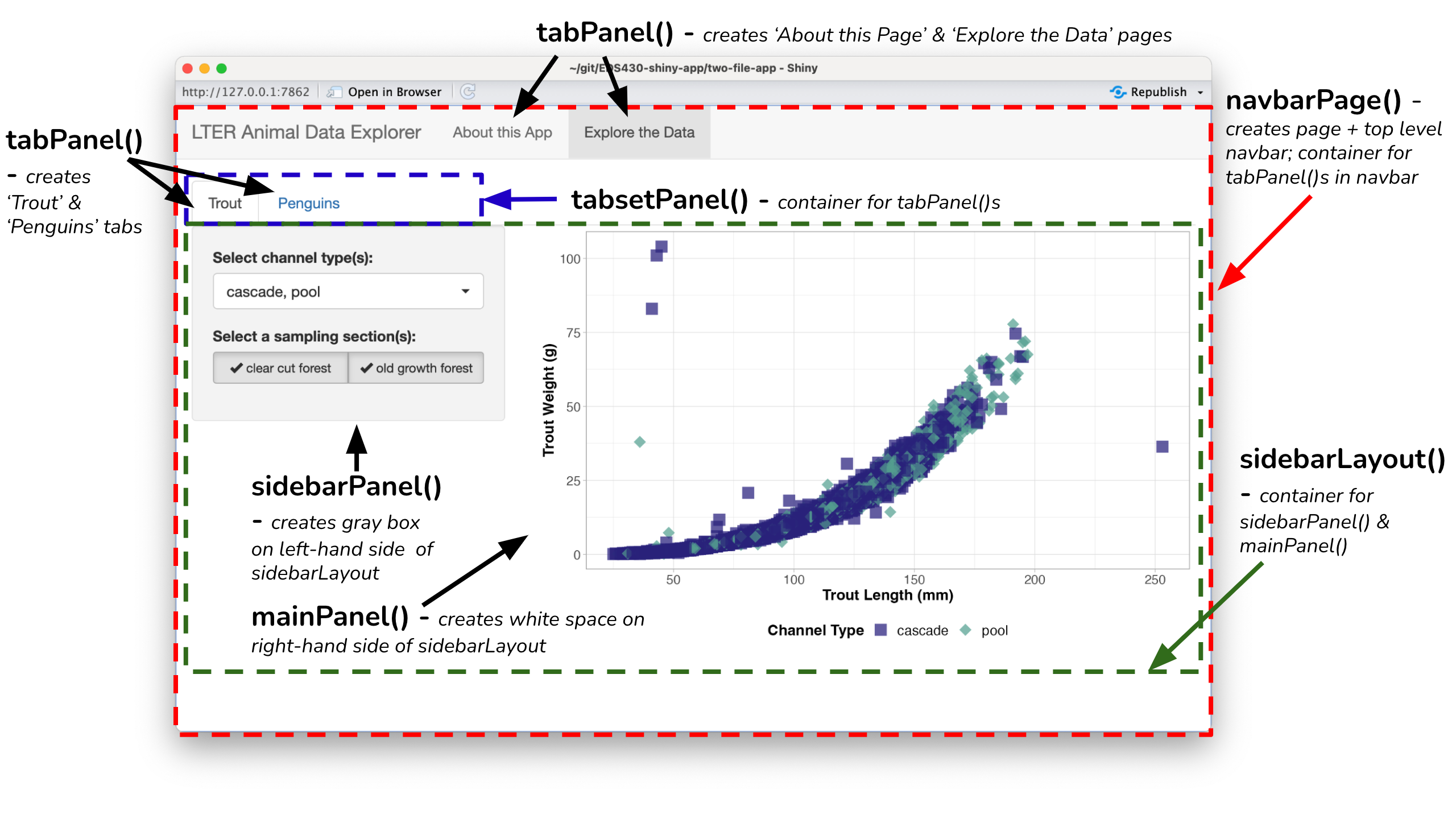
Layout functions provide the high-level visual structure of your app
Layouts are created using a hierarchy of function calls (typically) insidefluidPage(). Layouts often require a series functions – container functions establish the larger area within which other layout elements are placed. See a few minimal examples of layout functions on the following slides (though more exist!).
Some useful layout function pairings:
# sidebar for inputs & main area for outputs within the sidebarLayout() containersidebarLayout(sidebarPanel(),mainPanel())# multi-row fluid layout (add any number of fluidRow()s to a fluidPage())fluidRow(column(4, ...),column(8, ...))# tabPanel()s to contain HTML components (e.g. inputs/outputs) within the tabsetPanel() containertabsetPanel(tabPanel())# NOTE: can use navbarPage() in place of fluidPage(); creates a page with top-level navigation bar that can be used to toggle tabPanel() elementsnavbarPage(tabPanel())
Note: You can combine multiple layout function groups to really customize your UI – for example, you can create a navbar, include tabs, and also establish sidebar and main panel areas for inputs and outputs.
To create a page with a side bar and main area to contain your inputs and outputs (respectively), explore the following layout functions and read up on the sidebarLayout documentation:
fluidPage(titlePanel(# app title/description ),sidebarLayout(sidebarPanel(# inputs here ),mainPanel(# outputs here ) ))
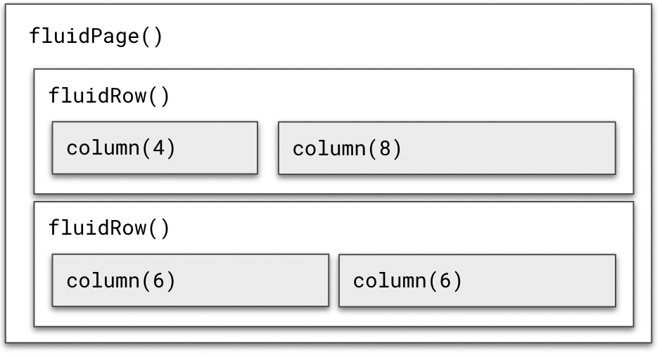
To create a page with multiple rows, explore the following layout functions and check out the fluid layout documentation. Note that each row is made up of 12 columns. The first argument of the column() function takes a value of 1-12 to specify the number of columns to occupy.
You may find that you eventually end up with too much content to fit on a single application page. Enter tabsetPanel() and tabPanel(). tabsetPanel() creates a container for any number of tabPanel()s. Each tabPanel() can contain any number of HTML components (e.g. inputs and outputs). Find the tabsetPanel documentation here and check out this example:
tabsetPanel(tabPanel("Tab 1", # an input# an output ),tabPanel("Tab 2"),tabPanel("Tab 3"))
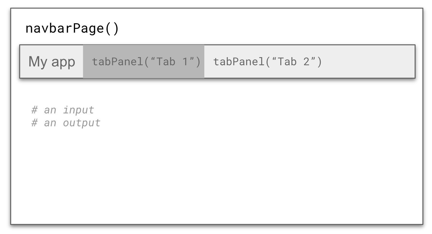
You may also want to use a navigation bar (navbarPage()) with different pages (created using tabPanel()) to organize your application. Read through the navbarPage documentation and try running the example below:
navbarPage(title ="My app",tabPanel(title ="Tab 1",# an input# an output ),tabPanel(title ="Tab 2"))
Overview of layout functions used in App #2
Important tips for success
Enable rainbow parentheses: Tools > Global Options > Code > Display > check Use rainbow parentheses
Add code comments at the start and end of each UI element: Even with rainbow parentheses, it can be easy to lose track or mistake what parentheses belong with which (see examples on follow slide)
Add placeholder text within your layout functions: Adding text, like "slider input will live here" and "plot output here" will help you better visualize what you’re working towards. It also makes it easier to navigate large UIs as you begin adding real inputs and outputs.
Use keyboard shortcuts to realign your code: Select all your code using cmd / ctrl + A, then realign using cmd / ctrl + I.
Build a navbar with two pages
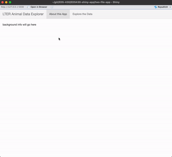
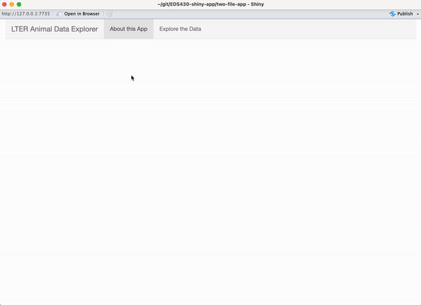
First, let’s build a UI that has a navigation bar with two tabs – one for background information and one to contain our data visualizations. To do this, we’ll use navbarPage() instead of fluidPage() to create our webpage.
~/two-file-app/ui.R
ui <-navbarPage(title ="LTER Animal Data Explorer",# (Page 1) intro tabPanel ----tabPanel(title ="About this App","background info will go here"# REPLACE THIS WITH CONTENT ), # END (Page 1) intro tabPanel# (Page 2) data viz tabPanel ----tabPanel(title ="Explore the Data","inputs and outputs will live here"# REPLACE THIS WITH CONTENT ) # END (Page 2) data viz tabPanel) # END navbarPage
Tip: Run your app often while building out your UI to make sure it’s looking as you’d expect!
Add two tabs to the “Explore the Data” page
Give your tabs the following titles: Trout and Penguins.
~/two-file-app/ui.R
ui <-navbarPage(title ="LTER Animal Data Explorer",# (Page 1) intro tabPanel ----tabPanel(title ="LTER Animal Data Explorer","background info will go here"# REPLACE THIS WITH CONTENT ), # END (Page 1) intro tabPanel# (Page 2) data viz tabPanel ----tabPanel(title ="Explore the Data",# tabsetPanel to contain tabs for data viz ----tabsetPanel(# trout tabPanel ----tabPanel(title ="Trout","trout data viz here"# REPLACE THIS WITH CONTENT ), # END trout tabPanel # penguin tabPanel ----tabPanel(title ="Penguins","penguin data viz here"# REPLACE THIS WITH CONTENT ) # END penguin tabPanel ) # END tabsetPanel ) # END (Page 2) data viz tabPanel) # END navbarPage
Add sidebar & main panels to the Trout tab
We’ll eventually place our input in the sidebar and output in the main panel.
~/two-file-app/ui.R
ui <-navbarPage(title ="LTER Animal Data Explorer",# (Page 1) intro tabPanel ----tabPanel(title ="About this App","background info will go here"# REPLACE THIS WITH CONTENT ), # END (Page 1) intro tabPanel# (Page 2) data viz tabPanel ----tabPanel(title ="Explore the Data",# tabsetPanel to contain tabs for data viz ----tabsetPanel(# trout tabPanel ----tabPanel(title ="Trout",# trout sidebarLayout ----sidebarLayout(# trout sidebarPanel ----sidebarPanel("trout plot input(s) go here"# REPLACE THIS WITH CONTENT ), # END trout sidebarPanel# trout mainPanel ----mainPanel("trout plot output goes here"# REPLACE THIS WITH CONTENT ) # END trout mainPanel ) # END trout sidebarLayout ), # END trout tabPanel # penguin tabPanel ----tabPanel(title ="Penguins","penguin data viz here"# REPLACE THIS WITH CONTENT ) # END penguin tabPanel ) # END tabsetPanel ) # END (Page 2) data viz tabPanel) # END navbarPage
Exercise 2: Add sidebar and main panels to the Penguins tab
I encourage you to type the code out yourself, rather than copy / paste!
Be sure to add text where your input / output will eventually be placed.
When you’re done, you app should look like this
See next slide for a solution!
Exercise 2: A solution
~/two-file-app/ui.R
ui <-navbarPage(title ="LTER Animal Data Explorer",# (Page 1) intro tabPanel ----tabPanel(title ="About this App","background info will go here"# REPLACE THIS WITH CONTENT ), # END (Page 1) intro tabPanel# (Page 2) data viz tabPanel ----tabPanel(title ="Animal Data Explorer",# tabsetPanel to contain tabs for data viz ----tabsetPanel(# trout tabPanel ----tabPanel(title ="Trout",# trout sidebarLayout ----sidebarLayout(# trout sidebarPanel ----sidebarPanel("trout plot input(s) go here"# REPLACE THIS WITH CONTENT ), # END trout sidebarPanel# trout mainPanel ----mainPanel("trout plot output goes here"# REPLACE THIS WITH CONTENT ) # END trout mainPanel ) # END trout sidebarLayout ), # END trout tabPanel # penguin tabPanel ----tabPanel(title ="Penguins",# penguin sidebarLayout ----sidebarLayout(# penguin sidebarPanel ----sidebarPanel("penguin plot input(s) go here"# REPLACE THIS WITH CONTENT ), # END penguin sidebarPanel# penguin mainPanel ----mainPanel("penguin plot output goes here"# REPLACE THIS WITH CONTENT ) # END penguin mainPanel ) # END penguin sidebarLayout ) # END penguin tabPanel ) # END tabsetPanel ) # END (Page 2) data viz tabPanel) # END navbarPage
Some important things to remember when building your UI’s layout:
try creating a rough sketch of your intended layout before hitting the keyboard (I like to think of this as UI layout “pseudocode”)
keeping clean code is important – we haven’t even any added any content yet and our UI is already >70 lines of code!
use rainbow parentheses, code comments and plenty of space between lines to keep things looking manageable and navigable
use the keyboard shortcut, command + I (Mac) or control + I (Windows), to align messy code – this helps put those off-alignment parentheses back where they belong
things can get out of hand quickly – add one layout section at a time, run your app to check that things look as you intend, then continue
Add data viz: First up, trout
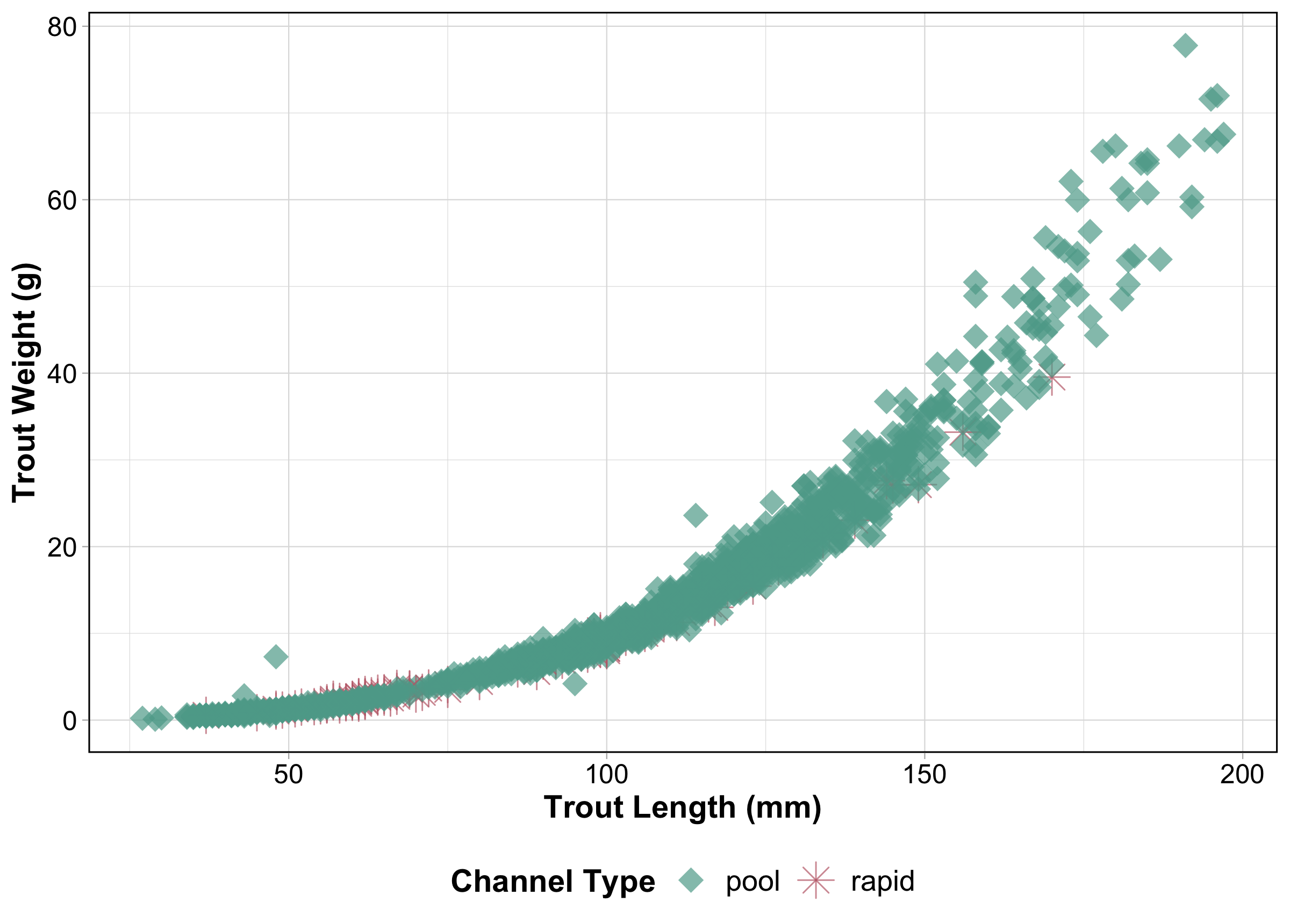
We’ll be using the and_vertebrates dataset from the {lterdatasampler} package to create our first reactive plot. These data contain coastal cutthroat trout (Oncorhynchus clarkii clarkii) lengths and weights collected in Mack Creek, Andrews Forest LTER. Original data can be found on the EDI Data Portal. Refer back to this slide to revisit our practice data wrangling & visualization script.
In addition to the {lterdatasampler} package, we’ll also be using the {tidyverse} for data wrangling / visualization, and the {shinyWidgets} package to add a pickerInput and a checkboxGroupInput to our app.
Import those three packages at the top of your global.R file
We can also do the bulk of our data wrangling here, rather than in the server. If we were reading in a data file (e.g. .csv), we would do that here too. Our new data object clean_trout, will now be available for us to call directly in our server (NOTE: we can copy our wrangling code over from our practice script).
~/two-file-app/global.R
# LOAD LIBRARIES ----library(shiny)library(tidyverse)library(shinyWidgets) library(lterdatasampler)# DATA WRANGLING ----# NOTE: if working with really large data, it is often beneficial to write your wrangled data to file, then read that file directly into `global.R`; this can help to increase your app's speedclean_trout <- and_vertebrates |>filter(species =="Cutthroat trout") |>select(sampledate, section, species, length_mm = length_1_mm, weight_g, channel_type = unittype) |>mutate(channel_type =case_when( channel_type =="C"~"cascade", channel_type =="I"~"riffle", channel_type =="IP"~"isolated pool", channel_type =="P"~"pool", channel_type =="R"~"rapid", channel_type =="S"~"step (small falls)", channel_type =="SC"~"side channel" )) |>mutate(section =case_when( section =="CC"~"clear cut forest", section =="OG"~"old growth forest" )) |>drop_na()
Add a pickerInput for selecting channel_type to your UI
The channel_type variable (originally called unittype – we updated the name when wrangling data) represents the type of water body (cascade, riffle, isolated pool, pool, rapid, step (small falls), or side channel) where data were collected. We’ll start by building a shinyWidgets::pickerInput() to allow users to filter data based on channel_type.
Reminder: When we designed our UI layout, we added a sidebarPanel to our Trout tab with the placeholder text "trout plot input(s) go here". Replace that text with the code for your pickerInput:
~/two-file-app/ui.R
# channel type pickerInput ----pickerInput(inputId ="channel_type_input", label ="Select channel type(s):",choices =unique(clean_trout$channel_type), # alternatively: choices = c("rapid", "cascade" ...)selected =c("cascade", "pool"),multiple =TRUE,options =pickerOptions(actionsBox =TRUE) # creates "Select All / Deselect All" buttons ) # END channel type pickerInput
Save and run your app – a functional pickerInput should now appear in your UI.
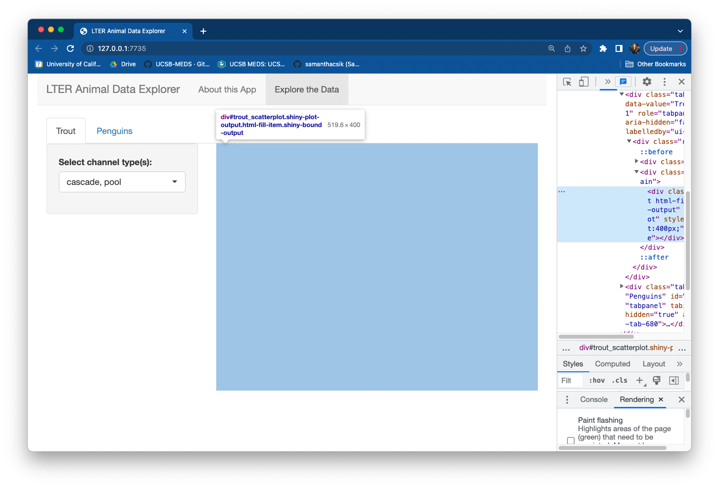
Add a plot output to your UI
Next, we need to create a placeholder in our UI for our trout scatterplot to live. Because we’ll be creating a reactive plot, we can use the plotOutput() function to do so.
Reminder: When we we designed our UI layout, we added a mainPanel to our Trout tab with the placeholder text "trout plot output goes here". Replace that text with the code for your plotOuput():
~/two-file-app/ui.R
plotOutput(outputId ="trout_scatterplot_output")
Save and run your app – it won’t look different at first glance, but inspecting your app in a browser window (using Chrome, right click > Inspect) will reveal a placeholder box for your plot output to eventually live:
Tell the server how to assemble pickerInput values into your plotOutput
Remember the three rules for building reactive outputs:(1) save objects you want to display to output$<id>, (2) build reactive objects using a render*() function, and (3) access input values with input$<id>:
~/two-file-app/server.R
server <-function(input, output) {# filter trout data ---- trout_filtered_df <-reactive({ clean_trout |>filter(channel_type %in%c(input$channel_type_input)) })# trout scatterplot ---- output$trout_scatterplot_output <-renderPlot({ggplot(trout_filtered_df(), aes(x = length_mm, y = weight_g, color = channel_type, shape = channel_type)) +geom_point(alpha =0.7, size =5) +scale_color_manual(values =c("cascade"="#2E2585", "riffle"="#337538", "isolated pool"="#DCCD7D","pool"="#5DA899", "rapid"="#C16A77", "step (small falls)"="#9F4A96","side channel"="#94CBEC")) +scale_shape_manual(values =c("cascade"=15, "riffle"=17, "isolated pool"=19,"pool"=18, "rapid"=8, "step (small falls)"=23,"side channel"=25)) +labs(x ="Trout Length (mm)", y ="Trout Weight (g)", color ="Channel Type", shape ="Channel Type") +myCustomTheme() }) } # END server
A couple notes / reminders:
If needed, reference your practice script to remind yourself how you planned to filter and plot your data
Reactive data frames need a set of parentheses, (), following the name of the df (see ggplot(trout_filtered_df() ...))
Saving your ggplot theme as a function in global.R makes it easy to build plots with a cohesive appearance (see code on following slide)
Save your custom ggplot theme to global.R
This allows us to easily add our theme as a layer to each of our ggplots. Bonus: If you decide to modify your plot theme, you only have to do so in one place.
Add a second input that will update the same output
You can have more than one input control the same output. Let’s now add a checkboxGroupButtons widget to our UI for selecting forest section (either clear cut forest or old growth forest). Check out the function documentation for more information on how to customize the appearance of your buttons.
Be sure to add the widget to the same sidebarPanel as our pickerInput (and separate them with a comma!):
~/two-file-app/ui.R
# trout plot sidebarPanel ----sidebarPanel(# channel type pickerInput ----pickerInput(inputId ="channel_type_input", label ="Select channel type(s):",choices =unique(clean_trout$channel_type),selected =c("cascade", "pool"),options =pickerOptions(actionsBox =TRUE),multiple =TRUE), # END channel type pickerInput# section checkboxGroupButtons ----checkboxGroupButtons(inputId ="section_input", label ="Select a sampling section(s):",choices =c("clear cut forest", "old growth forest"),selected =c("clear cut forest", "old growth forest"),individual =FALSE, justified =TRUE, size ="sm",checkIcon =list(yes =icon("check", lib ="font-awesome"), no =icon("xmark", lib ="font-awesome"))), # END section checkboxGroupInput ) # END trout plot sidebarPanel
Update your reactive df to also filter based on the new checkboxGroupInput
Return to your server to modify trout_filtered_df – our data frame needs to be updated based on both the pickerInput, which selects for channel_type, and the checkboxGrouptInput, which selects for forest section:
Run your app and try out your pickerInput & checkboxGrouptInput widgets!
Take a break
Up next: Adding in the penguins plot
05:00
Add data viz: Next up, penguins
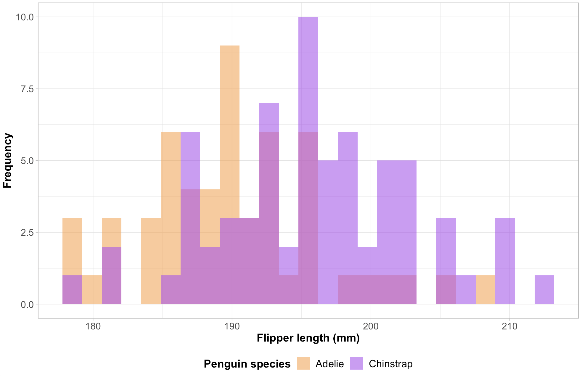
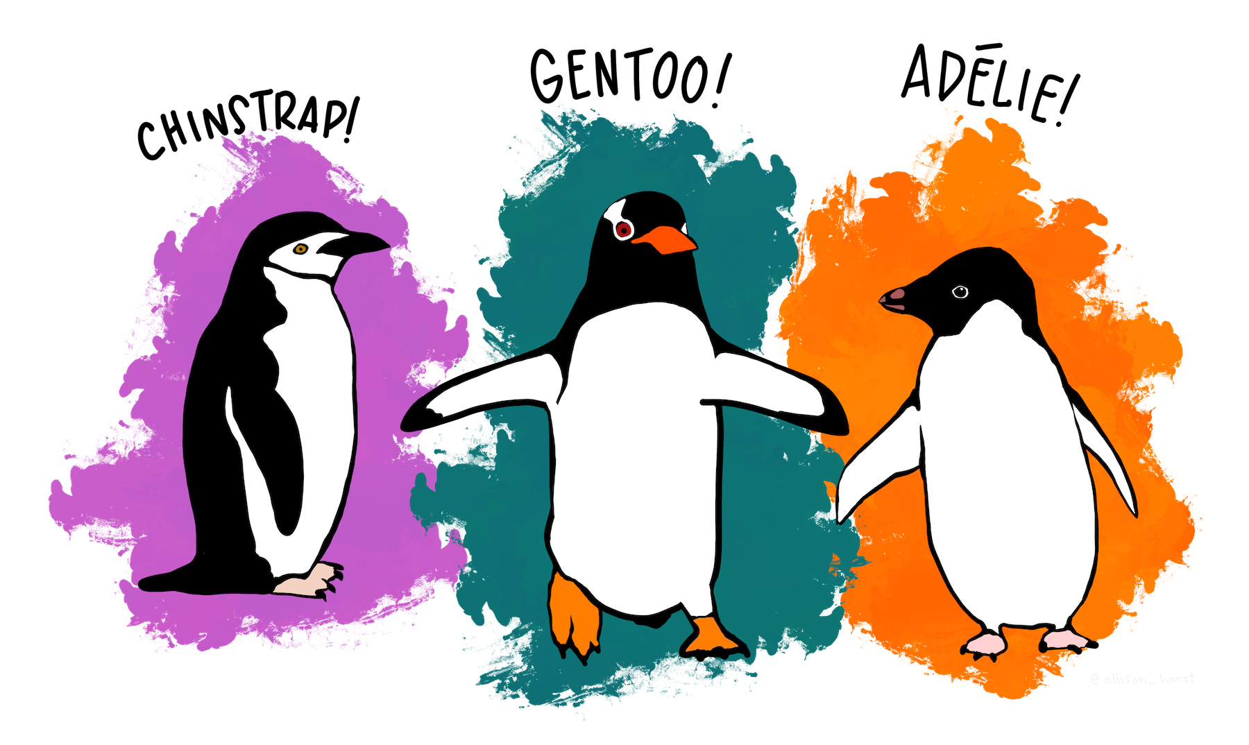
We’ll be using the penguins dataset from the {palmerpenguins} package to create our second reactive plot. These data contain penguin (genus Pygoscelis) body size measurements collected from three islands in the Palmer Archipelago, Antarctica, as part of the Palmer Station LTER. Original data can be found on the EDI Data Portal (Adélie data, Gentoo data, and Chinstrap data). Refer back to this slide to revisit our practice data wrangling & visualization script.
Exercise 3: Add a reactive plot to the ‘Penguins’ tab
Working alone or in groups, add a reactive histogram of penguin flipper lengths (using the penguins data set from the {palmerpenguins} package) to the Penguins tab. Your plot should have the following features and look like the example below, when complete:
data colored by penguin species
a shinyWidgets::pickerInput() that allows users to filter data based on island, and that includes buttons to Select All / Deselect All islands at once
a shiny::sliderInput() that allows users to change the number of histogram bins and that by default, displays a histogram with 25 bins
the two widgets should be placed in the sidebarPanel and the reactive histogram should be placed in the mainPanel of the Penguins tab
See next slide for some tips on getting started!
Exercise 3: Tips
Tips:
Remember to load the {palmerpenguins} package at the top of global.R so that your app can find the data
Add your widgets to the sidebarPanel and your plot output to the mainPanel of the Penguins tab – look for that placeholder text we added earlier to help place your new code in the correct spot within your UI!
Try changing the histogram bin number in your practice code script first, before attempting to make it reactive
And remember to follow the our three steps for building reactive outputs:
ui <-navbarPage(title ="LTER Animal Data Explorer",# (Page 1) intro tabPanel ----tabPanel(title ="About this App", ), # END (Page 1) intro tabPanel# (Page 2) data viz tabPanel ----tabPanel(title ="Explore the Data",# tabsetPanel to contain tabs for data viz ----tabsetPanel(# trout tabPanel ----tabPanel(title ="Trout",# trout plot sidebarLayout ----sidebarLayout(# trout plot sidebarPanel ----sidebarPanel(# channel type pickerInput ----pickerInput(inputId ="channel_type_input", label ="Select channel type(s):",choices =unique(clean_trout$channel_type),selected =c("cascade", "pool"),multiple =TRUE,options =pickerOptions(actionsBox =TRUE)), # END channel type pickerInput# # section checkboxGroupInput ----checkboxGroupButtons(inputId ="section_input", label ="Select a sampling section(s):",choices =c("clear cut forest", "old growth forest"),selected =c("clear cut forest", "old growth forest"),individual =FALSE, justified =TRUE, size ="sm",checkIcon =list(yes =icon("check", lib ="font-awesome"), no =icon("xmark", lib ="font-awesome"))), # END section checkboxGroupInput ), # END trout plot sidebarPanel# trout plot mainPanel ----mainPanel(plotOutput(outputId ="trout_scatterplot_output") ) # END trout plot mainPanel ) # END trout plot sidebarLayout ), # END trout tabPanel # penguin tabPanel ----tabPanel(title ="Penguins",# penguin plot sidebarLayout ----sidebarLayout(# penguin plot sidebarPanel ----sidebarPanel(# island pickerInput ----pickerInput(inputId ="penguin_island_input", label ="Select an island(s):",choices =c("Torgersen", "Dream", "Biscoe"),selected =c("Torgersen", "Dream", "Biscoe"),multiple =TRUE,options =pickerOptions(actionsBox =TRUE)), # END island pickerInput# bin number sliderInput ----sliderInput(inputId ="bin_num_input", label ="Select number of bins:",min =1, max =100, value =25) # END bin number sliderInput ), # END penguin plot sidebarPanel# penguin plot mainPanel ----mainPanel(plotOutput(outputId ="flipper_length_histogram_output") ) # END penguin plot mainPanel ) # END penguin plot sidebarLayout ) # END penguin tabPanel ) # END tabsetPanel ) # END (Page 2) data viz tabPanel) # END navbarPage
~/two-file-app/server.R
server <-function(input, output) {# filter for channel types ---- trout_filtered_df <-reactive({ clean_trout |>filter(channel_type %in%c(input$channel_type_input)) |>filter(section %in%c(input$section_input)) })# trout scatterplot ---- output$trout_scatterplot_output <-renderPlot({ggplot(trout_filtered_df(), aes(x = length_mm, y = weight_g, color = channel_type, shape = channel_type)) +geom_point(alpha =0.7, size =5) +scale_color_manual(values =c("cascade"="#2E2585", "riffle"="#337538", "isolated pool"="#DCCD7D","pool"="#5DA899", "rapid"="#C16A77", "step (small falls)"="#9F4A96","side channel"="#94CBEC")) +scale_shape_manual(values =c("cascade"=15, "riffle"=17, "isolated pool"=19,"pool"=18, "rapid"=8, "step (small falls)"=23,"side channel"=25)) +labs(x ="Trout Length (mm)", y ="Trout Weight (g)", color ="Channel Type", shape ="Channel Type") +myCustomTheme() })# filter for island ---- island_df <-reactive({ penguins |>filter(island %in% input$penguin_island_input) })# render the flipper length histogram ---- output$flipper_length_histogram_output <-renderPlot({ggplot(na.omit(island_df()), aes(x = flipper_length_mm, fill = species)) +geom_histogram(alpha =0.6, position ="identity", bins = input$bin_num_input) +scale_fill_manual(values =c("Adelie"="#FEA346", "Chinstrap"="#B251F1", "Gentoo"="#4BA4A4")) +labs(x ="Flipper length (mm)", y ="Frequency",fill ="Penguin species") +myCustomTheme() })} # END server
Take a break
Up next: we’ll finish up by adding some intro text to the landing page
05:00
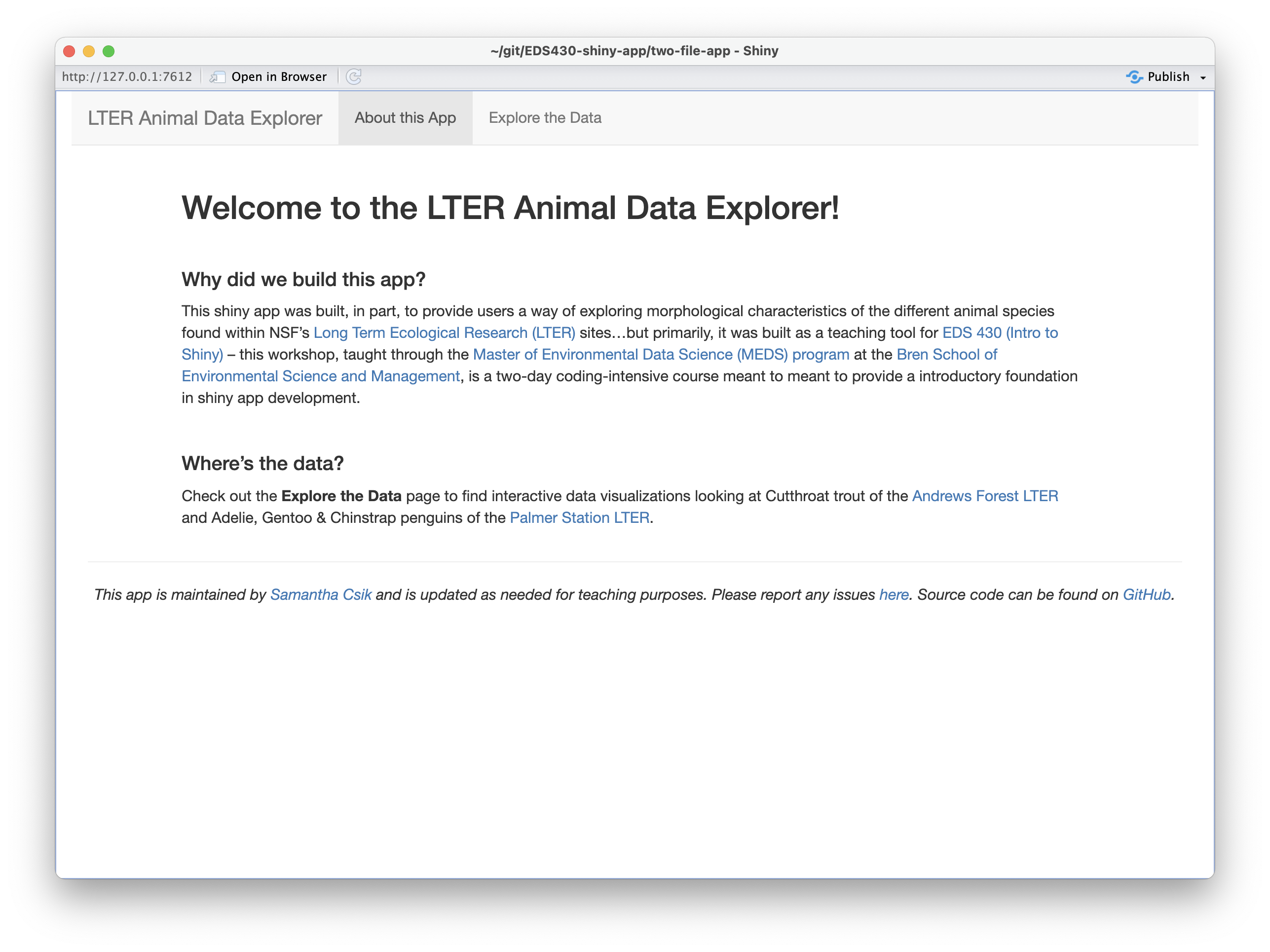
Add background / other important text
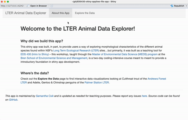
It’s usually valuable (and important) to provide some background information / context for your app – the landing page of your app can be a great place for this (but certainly doesn’t have to be where it lives). We’re going to add text to our app’s landing page (i.e. the About this App page) so that it looks like the example below:
Some important pieces for information to consider adding:
motivation for building the app
brief instructions for exploring the data
who maintains the app, where the code lives, how to submit issues / suggestions
Adding long text to the UI can get unruly
For example, I’ve added and formatted my landing page’s text directly in the UI using lots of nested tags – I’ve done this inside the tabPanel titled About this App (Note: I’ve formatted the layout of this page a bit using fluidRow and columns to create some white space around the edges. I’ve also created a faint gray horizontal line, using hr(), beneath which I added a footnote):
~/two-file-app/ui.R
ui <-navbarPage(title ="LTER Animal Data Explorer",# (Page 1) intro tabPanel ----tabPanel(title ="About this App",fluidRow(column(1),column(10, tags$h1("Welcome to the LTER Animal Data Explorer!"), tags$br(), tags$h2("Why did we build this app?"), tags$p("This shiny app was built, in part, to provide users a way of exploring morphological characteristics of the different animal species found within NSF's", tags$a(href ="https://lternet.edu/", "Long Term Ecological Research (LTER)"), "sites...but primarily, it was built as a teaching tool for", tags$a(href ="https://bren.ucsb.edu/courses/eds-430", "EDS 296 (Intro to Shiny)"), "-- this workshop, taught through the", tags$a(href ="https://ucsb-meds.github.io/", "Master of Environmental Data Science (MEDS) program"), "at the", tags$a(href ="https://bren.ucsb.edu/", "Bren School of Environmental Science and Management"), "is a two-day coding-intensive course meant to provide a introductory foundation in shiny app development."), tags$br(), tags$h2("Where's the data?"), tags$p("Check out the", tags$strong("Explore the Data"), "page to find interactive data visualizations looking at Cutthroat trout of the", tags$a(href ="https://andrewsforest.oregonstate.edu/", "Andrews Forest LTER"), "and Adélie, Gentoo & Chinstrap penguins of the", tags$a(href ="https://pallter.marine.rutgers.edu/", "Palmer Station LTER.")) ),column(1) ), # END fluidRowhr(),em("This app is maintained by", tags$a(href ="https://samanthacsik.github.io/", "Samantha Shanny-Csik"), "and is updated as needed for teaching purposes. Please report", tags$a(href ="https://github.com/samanthacsik/EDS-296-shiny-apps/issues", "any issues."), "Source code can be found on", tags$a(href ="https://github.com/samanthacsik/EDS-296-shiny-apps", "GitHub.")) ), # END (Page 1) intro tabPanel# (Page 2) data viz tabPanel ----tabPanel(title ="Explore the Data",# tabsetPanel to contain tabs for data viz ----tabsetPanel(# trout tabPanel ----tabPanel(title ="Trout",# trout plot sidebarLayout ----sidebarLayout(# trout plot sidebarPanel ----sidebarPanel(# channel type pickerInput ----pickerInput(inputId ="channel_type_input", label ="Select channel type(s):",choices =unique(clean_trout$channel_type),options =pickerOptions(actionsBox =TRUE),selected =c("cascade", "pool"),multiple =TRUE), # END channel type pickerInput# # section checkboxGroupInput ----checkboxGroupButtons(inputId ="section_input", label ="Select a sampling section:",choices =c("clear cut forest", "old growth forest"),selected =c("clear cut forest", "old growth forest"),individual =FALSE, justified =TRUE, size ="sm",checkIcon =list(yes =icon("ok", lib ="glyphicon"), no =icon("remove", lib ="glyphicon"))), # END section checkboxGroupInput ), # END trout plot sidebarPanel# trout plot mainPanel ----mainPanel(plotOutput(outputId ="trout_scatterplot_output") ) # END trout plot mainPanel ) # END trout plot sidebarLayout ), # END trout tabPanel # penguin tabPanel ----tabPanel(title ="Penguins",# penguin plot sidebarLayout ----sidebarLayout(# penguin plot sidebarPanel ----sidebarPanel(# island pickerInput ----pickerInput(inputId ="penguin_island_input", label ="Select an island:",choices =c("Torgersen", "Dream", "Biscoe"),options =pickerOptions(actionsBox =TRUE),selected =c("Torgersen", "Dream", "Biscoe"),multiple = T), # END island pickerInput# bin number sliderInput ----sliderInput(inputId ="bin_num_input", label ="Select number of bins:",value =25, max =100, min =1), # END bin number sliderInput ), # END penguin plot sidebarPanel# penguin plot mainPanel ----mainPanel(plotOutput(outputId ="flipper_length_histogram_output") ) # END penguin plot mainPanel ) # END penguin plot sidebarLayout ) # END penguin tabPanel ) # END tabsetPanel ) # END (Page 2) data viz tabPanel) # END navbarPage
Instead, use includeMarkdown()
Consider writing and styling long bodies of text in separate markdown (.md) files, then read them into your UI using includeMarkdown() (IMPORTANT: this requires the {markdown} package – be sure to add library(markdown) to your global.R file!). I recommend saving those .md files in a subdirectory named /text within your app’s directory (e.g. ~/two-file-app/text/mytext.md):
ui <-navbarPage(title ="LTER Animal Data Explorer",# (Page 1) intro tabPanel ----tabPanel(title ="About this App",# intro text fluidRow ----fluidRow(# use columns to create white space on sidescolumn(1),column(10, includeMarkdown("text/about.md")),column(1) ), # END intro text fluidRowhr(), # creates light gray horizontal line# footer text ----includeMarkdown("text/footer.md") ), # END (Page 1) intro tabPanel# (Page 2) data viz tabPanel ----tabPanel(title ="Explore the Data",# tabsetPanel to contain tabs for data viz ----tabsetPanel(# trout tabPanel ----tabPanel(title ="Trout",# trout plot sidebarLayout ----sidebarLayout(# trout plot sidebarPanel ----sidebarPanel(# channel type pickerInput ----pickerInput(inputId ="channel_type_input", label ="Select channel type(s):",choices =unique(clean_trout$channel_type),selected =c("cascade", "pool"),options =pickerOptions(actionsBox =TRUE),multiple =TRUE), # END channel type pickerInput# # section checkboxGroupInput ----checkboxGroupButtons(inputId ="section_input", label ="Select a sampling section:",choices =c("clear cut forest", "old growth forest"),selected =c("clear cut forest", "old growth forest"),individual =FALSE, justified =TRUE, size ="sm",checkIcon =list(yes =icon("ok", lib ="glyphicon"), no =icon("remove", lib ="glyphicon"))), # END section checkboxGroupInput ), # END trout plot sidebarPanel# trout plot mainPanel ----mainPanel(plotOutput(outputId ="trout_scatterplot_output") ) # END trout plot mainPanel ) # END trout plot sidebarLayout ), # END trout tabPanel# penguin tabPanel ----tabPanel(title ="Penguins",# penguin plot sidebarLayout ----sidebarLayout(# penguin plot sidebarPanel ----sidebarPanel(# island pickerInput ----pickerInput(inputId ="penguin_island_input", label ="Select an island:",choices =c("Torgersen", "Dream", "Biscoe"),selected =c("Torgersen", "Dream", "Biscoe"),options =pickerOptions(actionsBox =TRUE),multiple =TRUE), # END island pickerInput# bin number sliderInput ----sliderInput(inputId ="bin_num_input", label ="Select number of bins:",value =25, max =100, min =1), # END bin number sliderInput ), # END penguin plot sidebarPanel# penguin plot mainPanel ----mainPanel(plotOutput(outputId ="flipper_length_histogram_output") ) # END penguin plot mainPanel ) # END penguin plot sidebarLayout ) # END penguin tabPanel ) # END tabsetPanel ) # END (Page 2) data viz tabPanel) # END navbarPage
~/two-file-app/text/about.md
# Welcome to the LTER Animal Data Explorer!<br>## Why did we build this app?This shiny app was built, in part, to provide users a way of exploring morphological characteristics of the different animal species found within NSF's [Long Term Ecological Research (LTER)](https://lternet.edu/) sites...but primarily, it was built as a teaching tool for [EDS 296 (Intro to Shiny)](https://bren.ucsb.edu/courses/eds-430) -- this workshop, taught through the [Master of Environmental Data Science (MEDS) program](https://ucsb-meds.github.io/) at the [Bren School of Environmental Science and Management](https://bren.ucsb.edu/), is a two-day coding-intensive course meant to provide a introductory foundation in shiny app development.<br>## Where's the data? Check out the **Explore the Data** page to find interactive data visualizations looking at Cutthroat trout of the [Andrews Forest LTER](https://andrewsforest.oregonstate.edu/) and Adelie, Gentoo & Chinstrap penguins of the [Palmer Station LTER](https://pallter.marine.rutgers.edu/).
~/two-file-app/text/footer/md
*This app is maintained by [Samantha Shanny-Csik](https://samanthacsik.github.io/) and is updated as needed for teaching purposes. Please report [any issues](https://github.com/samanthacsik/EDS-296-shiny-apps/issues). Source code can be found on [GitHub](https://github.com/samanthacsik/EDS-296-shiny-apps).*
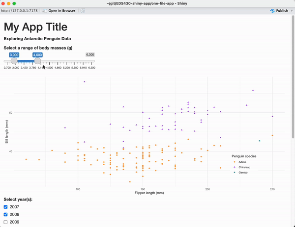
Run your app one more time to admire your beautiful creation!
Again, we have some UX/UI quirks to fix (most notably, blank plots when all widget options are deselected), which we’ll handle soon. But for now, we have a functioning app that we can practice deploying for the first time!
ui <-navbarPage(title ="LTER Animal Data Explorer",# (Page 1) intro tabPanel ----tabPanel(title ="About this App",# intro text fluidRow ----fluidRow(# use columns to create white space on sidescolumn(1),column(10, includeMarkdown("text/about.md")),column(1) ), # END intro text fluidRowhr(), # creates light gray horizontal line# footer text ----includeMarkdown("text/footer.md") ), # END (Page 1) intro tabPanel# (Page 2) data viz tabPanel ----tabPanel(title ="Explore the Data",# tabsetPanel to contain tabs for data viz ----tabsetPanel(# trout tabPanel ----tabPanel(title ="Trout",# trout plot sidebarLayout ----sidebarLayout(# trout plot sidebarPanel ----sidebarPanel(# channel type pickerInput ----pickerInput(inputId ="channel_type_input", label ="Select channel type(s):",choices =unique(clean_trout$channel_type), # alternatively, include vector of optionsselected =c("cascade", "pool"),multiple =TRUE,options =pickerOptions(actionsBox =TRUE)), # END channel type pickerInput# # section checkboxGroupInput ----checkboxGroupButtons(inputId ="section_input", label ="Select a sampling section(s):",choices =c("clear cut forest", "old growth forest"),selected =c("clear cut forest", "old growth forest"),individual =FALSE, justified =TRUE, size ="sm",checkIcon =list(yes =icon("check", lib ="font-awesome"), no =icon("xmark", lib ="font-awesome"))), # END section checkboxGroupInput ), # END trout plot sidebarPanel# trout plot mainPanel ----mainPanel(plotOutput(outputId ="trout_scatterplot_output") ) # END trout plot mainPanel ) # END trout plot sidebarLayout ), # END trout tabPanel # penguin tabPanel ----tabPanel(title ="Penguins",# penguin plot sidebarLayout ----sidebarLayout(# penguin plot sidebarPanel ----sidebarPanel(# island pickerInput ----pickerInput(inputId ="penguin_island_input", label ="Select an island(s):",choices =c("Torgersen", "Dream", "Biscoe"),selected =c("Torgersen", "Dream", "Biscoe"),options =pickerOptions(actionsBox =TRUE),multiple =TRUE), # END island pickerInput# bin number sliderInput ----sliderInput(inputId ="bin_num_input", label ="Select number of bins:",min =1, max =100, value =25), # END bin number sliderInput ), # END penguin plot sidebarPanel# penguin plot mainPanel ----mainPanel(plotOutput(outputId ="flipper_length_histogram_output") ) # END penguin plot mainPanel ) # END penguin plot sidebarLayout ) # END penguin tabPanel ) # END tabsetPanel ) # END (Page 2) data viz tabPanel) # END navbarPage
~/two-file-app/server.R
server <-function(input, output) {# filter for channel types ---- trout_filtered_df <-reactive({ clean_trout |>filter(channel_type %in%c(input$channel_type_input)) |>filter(section %in%c(input$section_input)) })# trout scatterplot ---- output$trout_scatterplot_output <-renderPlot({ggplot(trout_filtered_df(), aes(x = length_mm, y = weight_g, color = channel_type, shape = channel_type)) +geom_point(alpha =0.7, size =5) +scale_color_manual(values =c("cascade"="#2E2585", "riffle"="#337538", "isolated pool"="#DCCD7D","pool"="#5DA899", "rapid"="#C16A77", "step (small falls)"="#9F4A96","side channel"="#94CBEC")) +scale_shape_manual(values =c("cascade"=15, "riffle"=17, "isolated pool"=19,"pool"=18, "rapid"=8, "step (small falls)"=23,"side channel"=25)) +labs(x ="Trout Length (mm)", y ="Trout Weight (g)", color ="Channel Type", shape ="Channel Type") +myCustomTheme() })# filter for island ---- island_df <-reactive({ penguins |>filter(island %in% input$penguin_island_input) })# render the flipper length histogram ---- output$flipper_length_histogram_output <-renderPlot({ggplot(na.omit(island_df()), aes(x = flipper_length_mm, fill = species)) +geom_histogram(alpha =0.6, position ="identity", bins = input$bin_num_input) +scale_fill_manual(values =c("Adelie"="#FEA346", "Chinstrap"="#B251F1", "Gentoo"="#4BA4A4")) +labs(x ="Flipper length (mm)", y ="Frequency",fill ="Penguin species") +myCustomTheme() })} # END server
~/two-file-app/text/about.md
## Welcome to the LTER Animal Data Explorer!<br>## Why did we build this app?This shiny app was built, in part, to provide users a way of exploring morphological characteristics of the different animal species found within NSF's [Long Term Ecological Research (LTER)](https://lternet.edu/) sites...but primarily, it was built as a teaching tool for [EDS 296 (Intro to Shiny)](https://bren.ucsb.edu/courses/eds-430) -- this workshop, taught through the [Master of Environmental Data Science (MEDS) program](https://ucsb-meds.github.io/) at the [Bren School of Environmental Science and Management](https://bren.ucsb.edu/), is a two-day coding-intensive course meant to provide a introductory foundation in shiny app development.<br>## Where's the data? Check out the **Explore the Data** page to find interactive data visualizations looking at Cutthroat trout of the [Andrews Forest LTER](https://andrewsforest.oregonstate.edu/) and Adelie, Gentoo & Chinstrap penguins of the [Palmer Station LTER](https://pallter.marine.rutgers.edu/).
~/two-file-app/text/footer.md
*This app is maintained by [Samantha Shanny-Csik](https://samanthacsik.github.io/) and is updated as needed for teaching purposes. Please report [any issues](https://github.com/samanthacsik/EDS-296-shiny-apps/issues). Source code can be found on [GitHub](https://github.com/samanthacsik/EDS-296-shiny-apps).*