
Getting Started with Python
Pre-workshop prep
Please work through the following installations and configurations before attending the workshop:
NoteInstallation instructions (collapsed to save space)
1. Install Positron
Positron is the newest data science IDE (Integrated Development Environment) from Posit (the makers of RStudio) that combines the best features of RStudio (e.g. the data explorer, plots pane, etc.) with the flexibility and multi-language support of VS Code (a general-purpose IDE and a popular envrionment for writing Python code). Download and install Positron following these instructions.
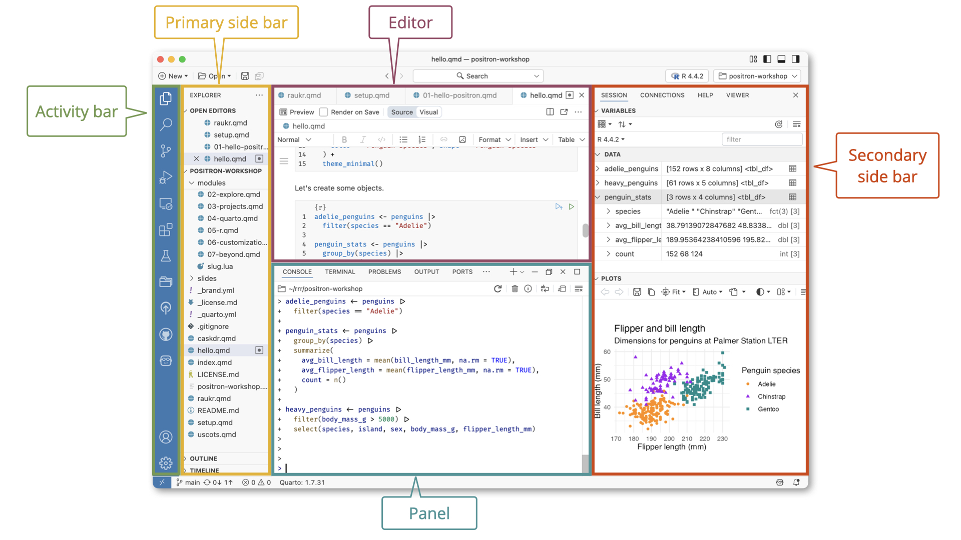
You can expand the features and capabilities of Positron by installing extensions. It already comes bundled with those needed for this workshop (Quarto, Jupyter notebooks), but know that you can install additional extensions, as needed, from the Extensions menu in the Activity Bar.
2. Install Miniforge3
conda is both a package installer and environment manager, built for data science work. We’ll learn more about it (and use it!) during the workshop. conda can be installed via several distributions (i.e. bundled collections of software that are packaged and distributed together for easy installation). The most well-known, Anaconda, bundles thousands of pre-installed packages you may never use, and requires accepting a commercial license for organizational use. Miniforge3 is a free, minimal alternative that gives you conda without the bloat, so you install only what you need. Installing Miniforge3 means you’ll receive a base environment containing Python, the conda package manager, and their essential dependencies. Follow the appropriate instructions, below, to install Miniforge3:
- Select the appropriate
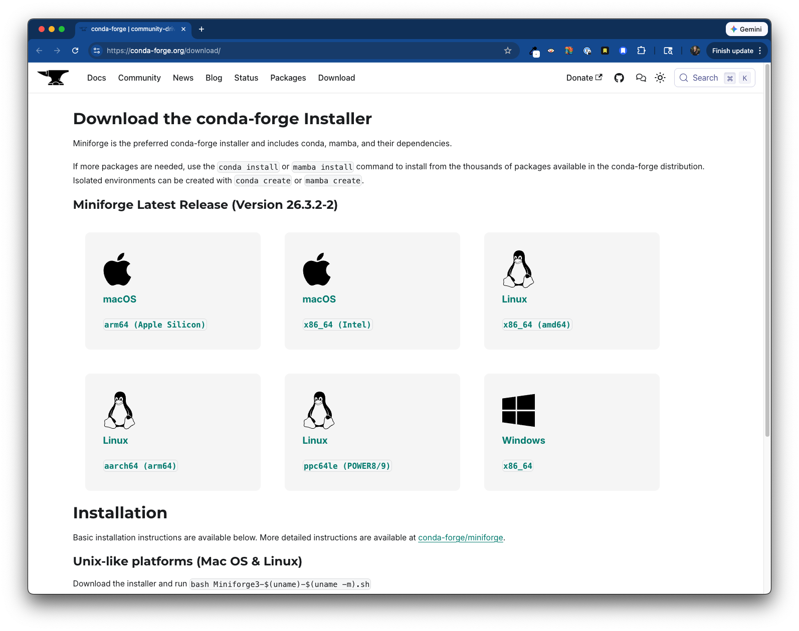
Miniforge3release from https://conda-forge.org/download/ to download a shell script (.shfile) for installation:
- Run your shell script in your Positron Terminal to install
Miniforge3. To do this:- Make sure you’re in your home directory. Check to see where you are in your computer by typing
pwd(“print working directory”) in your Terminal. If you’re already in your home directory, it should return something like,/Users/your-user-name. If you’re not in your home directory, you can jump there by typingcd ~(cdstands for “change directory”, and~is a shortcut for jumping home). - Move into your
Downloadsfolder, where your shell script currently lives, by typingcd Downloadsin your Terminal. - Run your shell script by typing
bash downloaded-file-name.sh(mine was named,Miniforge3-Darwin-arm64.sh) in your Terminal.
- Make sure you’re in your home directory. Check to see where you are in your computer by typing
- Follow the prompts in your Terminal to complete the installation:
- continue pressing ENTER until your reach the end of the license
- type
yesto accept the license terms - make sure to install it to your home directory (e.g.
Users/samanthacsik/miniforge3) when prompted - if asked if you want to update your shell profile to automatically initialize conda, type
yes
- Select the appropriate
Miniforge3release from https://conda-forge.org/download/ to download an executable (.exefile) for installation:
- Double click on the downloaded
.exeto begin the installation process. Follow the prompts:
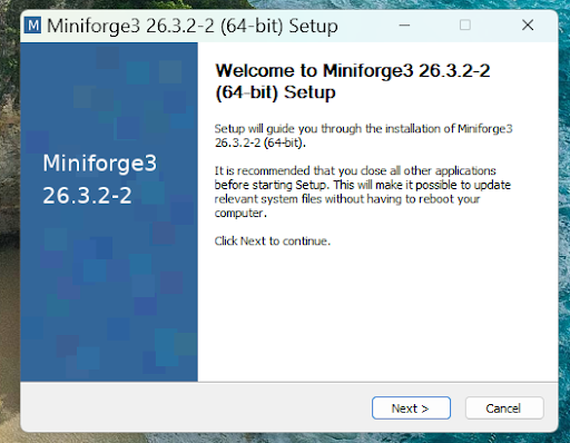
- Click next on the setup window:
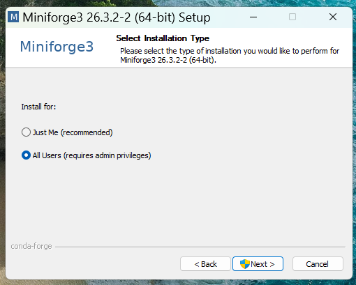
- Install for All Users, then click next:
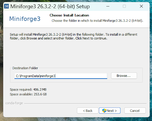
- Check that the destination folder is listed as
C:\ProgramData\miniforge3, then click next:
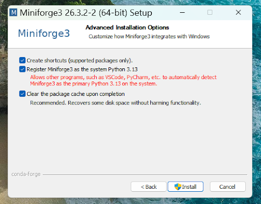
- Make sure all three Advanced Installation Options are selected, then click Install:
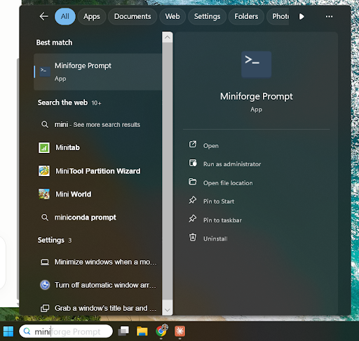
- Open up Miniforge Prompt:
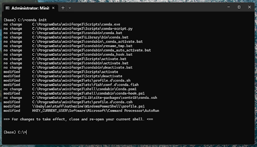
- Run
conda init:
Intro slides
We’ll start by familiarizing ourselves with some important terminology and concepts. You can access the Google Slides below:
Let’s write & run some Python code
Exercise 0: Create a new local project
Let’s start by creating a local repository (project) to store our work.
Open Positron and click on File > New Folder from Template… > Empty Project > give it a name (e.g. intro-python) and select where on your computer you’d like to save it to > click Create
Create two folders inside your project named
exercise1andexercise2. Click on the Explorer pane (it should already be open) > hover your mouse over your repository name until you see the New Folder… button > add your first folder, then repeat for the secondDownload a
.gitignoretemplate file from GitHub. A.gitignorefile is a plain text file used to tell Git which files or folders it should intentionally ignore and not track. While we won’t be using Git / GitHub to version control our files today, it’s helpful to be aware that the.gitignoretemplate for Python projects looks different than R projects. Run the following in your Positron Terminal:
Terminal
curl -O https://raw.githubusercontent.com/UCSB-MEDS/intro-to-python/refs/heads/main/.gitignore
TipcURL
cURL (i.e. Client URL) is an open-source command-line tool used by developers to transfer data to or from a server. It makes it easy to download a URL from a web server over HTTP. We’ll use this again in the next exercise!
Exercise 1: Run existing Python code
Sometimes you’ll receive Python code and an environment file (environment.yml or requirements.txt) from a collaborator (like the one in the folded chunk, below). In this exercise, you will reproduce an environment and run a Python script.
Note
environment.yml
environment.yml is a text file that specifies a conda environment’s name, channels to download from, and package dependencies. It’s similar to the requirements.txt file that’s used with venv (a virtual environment manager used in conjunction with pip).
environment.yml
name: cmip6-env
channels:
  - conda-forge
  - defaults
dependencies:
  - python=3.11
  - intake
  - intake-esm
  - s3fs
  - xarray
  - zarr
  - matplotlib
  - numpy
  - pandas
  - jupyter
- ipykernel- Download the
environment.ymland intro-to-python.ipynb from GitHub and save them to your project directory. Do this in the Terminal by running:
Terminal
# Download the environment.yml
curl -O https://raw.githubusercontent.com/UCSB-MEDS/intro-to-python/main/exercises/environment.yml

# Download the intro-to-python.ipynb notebook
curl -O https://raw.githubusercontent.com/UCSB-MEDS/intro-to-python/main/exercises/intro-to-python.ipynb- Once downloaded, you can drag and drop these files into your
exercise1/folder
- Create the
cmip6-envconda environment from our downloadedenvironment.ymlfile:
Terminal
conda env create -f exercise1/environment.yml- Activate the environment. You’ll want to make sure you’re in your correct environment (you should see
(cmip6-env)at the start of your command line whencmip6-envis correctly activated) before installing packages:
Terminal
conda activate cmip6-env- Register
cmip6-envas a Jupyter kernel so it’s available as a notebook interpreter:
Terminal
python -m ipykernel install --user --name cmip6-env --display-name "Python (cmip6-env)"Open
intro-to-python.ipynb(in Positron) and selectcmip6-envas your interpreter. Click the interpreter selector in the top right of the Jupyter Notebook and choosePython (cmip6-env). You may need to restart Positron to find your kernel. Shut down Positron entirely > reopen Positron > reopen your project by clicking the folder button (top right corner of Positron) and selecting your project > open your interpreter.Run through all the cells in the Jupyter Notebook (they should run!).
Exercise 2: Translating R to Python
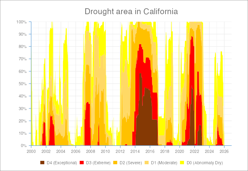
Let’s say you already have some R code for reproducing the US Drought Monitor’s “Drought area in California” visualization, and you’d like to translate it to Python:
NoteExpand for R code
##~~~~~~~~~~~~~~~~~~~~~~~~~~~~~~~~~~~~~~~~~~~~~~~~~~~~~~~~~~~~~~~~~~~~~~~~~~~~~~
##                                    setup                                 ----
##~~~~~~~~~~~~~~~~~~~~~~~~~~~~~~~~~~~~~~~~~~~~~~~~~~~~~~~~~~~~~~~~~~~~~~~~~~~~~~

#..........................load packages.........................
library(tidyverse)

#..........................import data...........................
drought <- read_csv(here::here("data", "drought.csv"))

##~~~~~~~~~~~~~~~~~~~~~~~~~~~~~~~~~~~~~~~~~~~~~~~~~~~~~~~~~~~~~~~~~~~~~~~~~~~~~~
##                            wrangle drought data                          ----
##~~~~~~~~~~~~~~~~~~~~~~~~~~~~~~~~~~~~~~~~~~~~~~~~~~~~~~~~~~~~~~~~~~~~~~~~~~~~~~

drought_clean <- drought |>

  # pivot table to be in tidy form ----
  pivot_longer(cols = none:d4, names_to = "drought_lvl", values_to = "area_pct") |>

  # select cols of interest & update names for clarity (as needed) ----
  select(start_date, state_abb, drought_lvl, area_pct) |>

  # coerce start_date to date ----
  mutate(start_date = mdy(start_date)) |>

  # add drought level conditions names ----
  mutate(drought_lvl_long = factor(drought_lvl,
                                   levels = c("d4", "d3", "d2", "d1", "d0", "none"),
                                   labels = c("D4 (Exceptional)", "D3 (Extreme)",
                                       "D2 (Severe)", "D1 (Moderate)",
                                       "D0 (Abnormaly Dry)",
                                       "No Drought"))) |>

  # reorder cols ----
  relocate(start_date, state_abb, drought_lvl, drought_lvl_long, area_pct) |>

  # remove drought_lvl "none" & filter for just CA ----
  filter(drought_lvl != "none",
         state_abb == "CA") |>

##~~~~~~~~~~~~~~~~~~~~~~~~~~~~~~~~~~~~~~~~~~~~~~~~~~~~~~~~~~~~~~~~~~~~~~~~~~~~~~
##       create stacked area plot of CA drought conditions through time     ----
##~~~~~~~~~~~~~~~~~~~~~~~~~~~~~~~~~~~~~~~~~~~~~~~~~~~~~~~~~~~~~~~~~~~~~~~~~~~~~~

# initialize ggplot ----
ggplot(drought_clean, mapping = aes(x = start_date, y = area_pct, fill = drought_lvl_long)) +

  # reverse order of groups so level D4 is closest to x-axis ----
  geom_area(position = position_stack(reverse = TRUE)) +

  # update colors to match US Drought Monitor ----
  # (colors identified using ColorPick Eyedropper extension on the original USDM data viz)
  scale_fill_manual(values = c("#853904", "#FF0000", "#FFC100", "#FFD965", "#FFFF00")) +

  # set x-axis breaks & remove padding between data and x-axis ----
  scale_x_date(breaks = scales::breaks_pretty(n = 13),
               limits = as.Date(c("2000-01-01", "2026-12-31")),
               expand = c(0,0)) +

  # set y-axis breaks & remove padding between data and y-axis & convert values to percentages ----
  scale_y_continuous(breaks = seq(0, 100, by = 10),
                     expand = c(0, 0),
                     labels = scales::label_percent(scale = 1)) +

  # add title ----
  labs(title = "Drought area in California") +

  # set theme minimal (includes major/minor grid lines, no axes) ----
  theme_minimal() +

  # fine-tune adjustments to plot theme ----
  theme(

    # update axis lines & ticks color ----
    axis.line = element_line(color = "#5A9CD6"),
    axis.ticks = element_line(color = "#5A9CD6"),

    # adjust length of axis ticks ----
    axis.ticks.length = unit(.2, "cm"),

    # center plot title ----
    plot.title = element_text(hjust = 0.5, color = "#686868", size = 20,
                              margin = margin(t = 10, r = 0, b = 15, l = 0)),

    # remove axis & legend titles ----
    axis.title = element_blank(),
    legend.title = element_blank(),

    # axis text color & size ----
    axis.text = element_text(color = "#686868", size = 10),
    legend.text = element_text(color = "#686868", size = 10),

    # move legend below plot ----
    legend.position = "bottom",
    legend.direction = "horizontal",
    legend.key.width = unit(0.4, "cm"),
    legend.key.height = unit(0.25, "cm"),

    # update plot background color & plot margins ----
    plot.background = element_rect(color = "#686868"),
    plot.margin = margin(t = 10, r = 40, b = 10, l = 40)
  )
- Download the necessary data and save it to
exercise2/data/(you’ll need to create adata/folder insideexericse2/then drag and dropdrought.csvinto it):
Terminal
curl -O https://raw.githubusercontent.com/UCSB-MEDS/intro-to-python/refs/heads/main/data/drought.csv- Let’s try to use claude.ai (or your preferred GenAI chatbot) to translate our R code into Python code. Try sharing the R code, above, along with the prompt,
Translate this R code into Python code using pandas for the data wrangling and plotnine for the data viz
TipTell your AI tool which Python packages you want to use
Check out this slide for Python equivalents to your favorite R packages.
- Add a new Python script named,
drought.pyto yourexercise2/folder and copy the AI-generated code into it. Yours may look a bit different than ours (and everyone else’s around you).
NoteExpand for AI-generated Python code
import pandas as pd
from plotnine import *

# ── Load data ──────────────────────────────────────────────────────────────────
drought = pd.read_csv("data/drought.csv")

# ── Wrangle ────────────────────────────────────────────────────────────────────
drought_clean = (
    drought
    # pivot to tidy form
    .melt(
        id_vars=[c for c in drought.columns if c not in ["none", "d0", "d1", "d2", "d3", "d4"]],
        value_vars=["none", "d0", "d1", "d2", "d3", "d4"],
        var_name="drought_lvl",
        value_name="area_pct",
    )
    # select cols of interest
    [["start_date", "state_abb", "drought_lvl", "area_pct"]]
    # coerce start_date to date
    .assign(
        start_date=lambda df: pd.to_datetime(df["start_date"]),
        drought_lvl_long=lambda df: pd.Categorical(
            df["drought_lvl"],
            categories=["d4", "d3", "d2", "d1", "d0"],
            ordered=True,
        ).rename_categories({
            "d4": "D4 (Exceptional)",
            "d3": "D3 (Extreme)",
            "d2": "D2 (Severe)",
            "d1": "D1 (Moderate)",
            "d0": "D0 (Abnormally Dry)",
        }),
    )
    # filter out "none" drought level and keep only CA
    .query("drought_lvl != 'none' and state_abb == 'CA'")
    .dropna(subset=["drought_lvl_long"])
)

# ── Plot ───────────────────────────────────────────────────────────────────────
(
    ggplot(drought_clean, aes(x="start_date", y="area_pct", fill="drought_lvl_long"))
    + geom_area(position=position_stack(reverse=True))
    + scale_fill_manual(
        values=["#853904", "#FF0000", "#FFC100", "#FFD965", "#FFFF00"]
    )
    + scale_x_datetime(
        breaks=date_breaks("2 years"),
        date_labels="%Y",
        limits=(pd.Timestamp("2000-01-01"), pd.Timestamp("2026-12-31")),
        expand=(0, 0),
    )
    + scale_y_continuous(
        breaks=range(0, 101, 10),
        expand=(0, 0),
        labels=lambda lst: [f"{v}%" for v in lst],
    )
    + labs(title="Drought area in California")
    + theme_minimal()
    + theme(
        axis_line=element_line(color="#5A9CD6"),
        axis_ticks=element_line(color="#5A9CD6"),
        axis_ticks_length=0.2,
        plot_title=element_text(ha="center", color="#686868", size=20,
                                margin={"t": 10, "b": 15}),
        axis_title=element_blank(),
        legend_title=element_blank(),
        axis_text=element_text(color="#686868", size=10),
        legend_text=element_text(color="#686868", size=10),
        legend_position="bottom",
        legend_direction="horizontal",
        legend_key_width=12,
        legend_key_height=8,
        plot_background=element_rect(color="#686868"),
        plot_margin=0.1,
    )
)- Create a new
condaenvironment calleddrought-envwith Python 3.11. While Python 3.13 is the latest version, many packages commonly used for environmental data science work haven’t been updated to support it yet, so we recommend using 3.11 to avoid compatibility issues:
Terminal
conda create -n drought-env python=3.11- Activate your
drought-envenvironment:
Terminal
conda activate drought-env- Install the necessary packages to your
drought-envfrom theconda-forgechannel (reminder: conda-forge is a large repository of community-maintained Python packages):
Terminal
conda install -c conda-forge pandas plotnine- Optionally, export your environment to an
environment.ymlfile so others can reproduce it. Use the--from-historyflag to export only the packages you explicitly installed, rather than all of their dependencies. This makes the file more portable across operating systems; instead of locking in your machine’s specific dependencies, it lets conda resolve the right ones for each user’s OS.
Terminal
conda env export --from-history > exercise2/environment.ymlRestart Positron, then select your interpreter by clicking the Interpreter Picker (top right corner of Positron) > click New Console Session… > choose the Python 3.11.14 (Conda: drought-env) interpreter.
Try running your
drought.pyscript. Your code will likely not run without some manual updates. Things to try / look out for:
- it’s helpful to run your code line-by-line
- make sure the file path for reading in your data is correct
- check out your df in Positron’s data viewer by running
%view drought_cleanin your console - try commenting out sections of code to get things running (even if it’s not perfect)
- ask AI to help interpret error messages
NoteExpand for manually-adjusted Python code
import pandas as pd
from plotnine import *

# ── Load data ──────────────────────────────────────────────────────────────────
1drought = pd.read_csv("exercise2/data/drought.csv")

# ── Wrangle ────────────────────────────────────────────────────────────────────
drought_clean = (
    drought
    # pivot to tidy form
    .melt(
        id_vars=[c for c in drought.columns if c not in ["none", "d0", "d1", "d2", "d3", "d4"]],
        value_vars=["none", "d0", "d1", "d2", "d3", "d4"],
        var_name="drought_lvl",
        value_name="area_pct",
    )
    # select cols of interest
    [["start_date", "state_abb", "drought_lvl", "area_pct"]]
    # coerce start_date to date
    .assign(
        start_date=lambda df: pd.to_datetime(df["start_date"]),
        drought_lvl_long=lambda df: pd.Categorical(
            df["drought_lvl"],
            categories=["d4", "d3", "d2", "d1", "d0"],
            ordered=True,
        ).rename_categories({
            "d4": "D4 (Exceptional)",
            "d3": "D3 (Extreme)",
            "d2": "D2 (Severe)",
            "d1": "D1 (Moderate)",
            "d0": "D0 (Abnormally Dry)",
        }),
    )
    # filter out "none" drought level and keep only CA
    .query("drought_lvl != 'none' and state_abb == 'CA'")
    .dropna(subset=["drought_lvl_long"])
)

# ── Plot ───────────────────────────────────────────────────────────────────────
(
    ggplot(drought_clean, aes(x="start_date", y="area_pct", fill="drought_lvl_long"))
    + geom_area(position=position_stack(reverse=True))
    + scale_fill_manual(
        values=["#853904", "#FF0000", "#FFC100", "#FFD965", "#FFFF00"]
    )
2    # + scale_x_datetime(
    #     breaks=date_breaks("2 years"),
    #     date_labels="%Y",
    #     limits=(pd.Timestamp("2000-01-01"), pd.Timestamp("2026-12-31")),
    #     expand=(0, 0),
    # )
    + scale_y_continuous(
        breaks=range(0, 101, 10),
        expand=(0, 0),
        labels=lambda lst: [f"{v}%" for v in lst],
    )
    + labs(title="Drought area in California")
    + theme_minimal()
    + theme(
        axis_line=element_line(color="#5A9CD6"),
        axis_ticks=element_line(color="#5A9CD6"),
        axis_ticks_length=0.2,
        plot_title=element_text(ha="center", color="#686868", size=20,
                                margin={"t": 10, "b": 15}),
        axis_title=element_blank(),
        legend_title=element_blank(),
        axis_text=element_text(color="#686868", size=10),
        legend_text=element_text(color="#686868", size=10),
        legend_position="bottom",
        legend_direction="horizontal",
        legend_key_width=12,
        legend_key_height=8,
        plot_background=element_rect(color="#686868"),
        plot_margin=0.1,
    )
)- 1
-
Updated the file path (our working directory is the project root, rather than where
drought.pylives) - 2
-
Running the code line-by-line reveals a
NameError: name 'date_breaks' is not defined.when we add in these lines of code. Asking claude.ai to explain the error helps us understand thatdate_breaksisn’t exported byfrom plotnine import *, but rather lives inmizani, the underlying scales/formatting dependency. It can be installed viaconda install -c conda-forge mizani. For now, we chose to comment out these lines of code to first get a working plot.
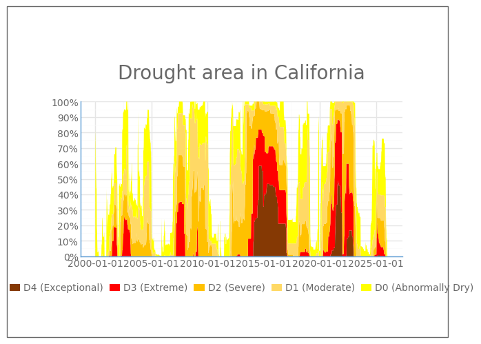
There are certainly a few more updates we should make to polish up this data viz, including:
- setting the x-axis breaks to something a bit cleaner (ideally, years)
- making sure the legend doesn’t spill outside of our plot
We don’t have time to do that today, but we encourage you to give it a try yourself!
Contribute
Have suggestions for improving these materials? File an issue on GitHub.