An iterative approach to streamlining your analytical workflows using functions and for loops

Author

Sam Csik

Published

April 14, 2023

By now, you may have heard instructors or online resources quote the saying, “If you’ve copied a block of code more than twice, you should probably consider writing a function.”

As your analyses get longer and more complex, the chances that you’ll benefit from writing functions will also increase – many times, this is to minimize the amount of code you need to copy/paste, but writing functions can also help to make your code:

more navigable (e.g. by partitioning your code and functions into separate files)
more readable (e.g. creating human-readable function names that tell a user exactly what to expect)
less prone to errors (e.g. less copying/pasting large code chunks means less opportunity to introduce bugs)

Iteration (i.e. performing the same operation on multiple inputs, e.g. multiple data sets, columns, etc.) is another tool for reducing duplication – for loops are one approach for performing iterative tasks. Together, both functions and for loops provide a powerful means to streamlining your analytical pipelines.

However, whether you’re a new learner or seasoned programmer, it can sometimes feel overwhelming to know exactly where to start – especially when you have an end goal that builds additional complexity/flexibility into your functions and for loops. Taking an iterative approach to building out your code can help make this process clearer, less daunting, and more fun.

This document walks through my own iterative process for writing a couple functions and for loops to clean and visualize multiple, similar data sets. The way I’ve written this code is certainly not the only way (and likely not even the most optimized way), but I hope that by stepping through how I slowly build out my functions to be more flexible and user-friendly, it might help demonstrate an iterative workflow that I find particularly effective.

How is this document organized?

This workshop is indended to be taught in-person

I’ll be doing a lot of writing code, then testing code, then adding a bit more code, rinsing, and repeating. That can be a bit hard to capture in an instructional document, but I’ve done my best to outline my iterative steps here for folks to refer back to, as-needed.

Sections

This document follows just one case study – creating functions and for loops for processing and visualizing ocean temperature data from a few Santa Barbara Coastal LTER rocky reef sites. I do this in three “Stages”, each of which includes multiple steps/code versions:

Stage 1: Clean and plot one data set – always my first step when beginning any analysis

this is a standard workflow that includes reading in the data, then cleaning and plotting at least one data set (I include these steps for all three data sets, for reference…this involves lots of copying and pasting large chunks of code!)

Stage 2: Write functions to clean & plot your data – getting a little fancier by turning long, repeated code chunks into functions

Here I create two separate functions, one to clean data and one to plot data – for each, I take a super iterative approach (i.e. I start by creating a relatively simple function (that works!), then build in more flexibility/complexity)

Stage 3: Write for loops to read in, clean, and plot all your data – streamline processing all of our data sets using less code

Once I’ve created functions that help to reduce the code needed for processing and plotting my data, I write a few for loops to read in, clean, and plot all files (while this may seem a bit silly for just three files, imagine having to process/plot dozens or more!). Again, I do this in a few separate steps so I can ensure each small piece works before adding in the next bit.

See what I’m Googling!

I realize that oftentimes, these carefully curated workshop materials may mask the amount of Googling / trial and error / general frustrations that I myself experience when building instructional content – I do a lot of Googling, and don’t know most of what I end up teaching off the top of my head. In an attempt to better normalize Googling for code help, I began saving some of the resources I referenced – they’re linked and noted with the symbol. Disclaimer: I only thought to do this about half-way through, so the amount of reference materials is severely underestimated (just know that I’ve either had to look up to remind myself how to do most things, or do some serious digging to learn how to do something for the first time). I’ll try to be more consistent about including these little side notes moving forward!

Check out the new Quarto code annotations feature!

Line-based code annotations are a new feature of Quarto version 1.3, and I think they’re pretty nifty. Find numbered explanations beneath particular code chunks – clicking on a number will highlight the corresponding line of code. You can learn more about using annotations here.

About the Data

The Santa Barbara Coastal Long Term Ecological Research (SBC LTER) site was established in 2000 and is located in Santa Barbara’s coastal zone, where ocean currents and climate are highly variable with season and longer-term cycles. A number of kelp forest/rocky reef sites exist, where long-term data collection occurs using a variety of methods, including both repeated surveys and moored instrumentation. Today, we’ll be exploring ocean temperature data, collected via moored instrumentation (CTDs), from just three of these sites: Alegria Reef, Mohwak Reef, and Carpinteria Reef.

Raw data are available for download on the EDI Data Portal:

Alegria Reef: https://portal.edirepository.org/nis/mapbrowse?packageid=knb-lter-sbc.2008.14
Mohawk Reef: https://doi.org/10.6073/pasta/cbe43646b801bf6ee5231c301ea23f51
Carpinteria Reef: https://portal.edirepository.org/nis/mapbrowse?packageid=knb-lter-sbc.2004.26

Setup

create and clone a GitHub repository (be sure to add a .gitignore file)
download the data – these data are publicly available via the EDI Data Portal, but I’ve also added the necessary files to Google Drive for download here – these are large data files and take a few minutes to download; be sure to unzip the files once downloaded
add a subdirectory called /data; move your unzipped raw_data folder into the /data subdirectory; your folder structure should now look like: your-repo/data/raw_data
add your /raw_data folder to your .gitignore file so that you don’t accidentally try pushing it to GitHub (these data files are far too large for that!) – to do so, scroll to the bottom of your .gitignore, type the following, data/raw_data/, and save; you can push this modified .gitignore file to GitHub now, if you’d like

Stage 1: Clean and plot one data set

Copying, pasting, and slightly updating code to clean and process multiple similarly-structured data sets is certainly the slowest and most prone-to-errors workflow. However, (in my honest opinion) it’s almost always critical to being by processing one data set on it’s own before attempting to write a function to do so.

Let’s start by doing that here.

Note

I’ll be writing the following code in a script called, no_functions_pipeline.R, which I’ll save to my repo’s root directory.

i. Load libraries

library(tidyverse)
library(chron)
library(naniar)
library(ggridges)

ii. Import raw data

Either download from the Environmental Data Portal (EDI) directly:

# ale <- read_csv("https://portal.edirepository.org/nis/dataviewer?packageid=knb-lter-sbc.2008.14&entityid=15c25abf9bb72e2017301fa4e5b2e0d4")
# mko <- read_csv("https://portal.edirepository.org/nis/dataviewer?packageid=knb-lter-sbc.2007.16&entityid=02629ecc08a536972dec021f662428aa")
# car <- read_csv("https://portal.edirepository.org/nis/dataviewer?packageid=knb-lter-sbc.2004.26&entityid=1d7769e33145ba4f04aa0b0a3f7d4a76")

Or read in the downloaded files from data/raw_data/:

alegria <- read_csv(here::here("data", "raw_data", "alegria_mooring_ale_20210617.csv"))
mohawk <- read_csv(here::here("data", "raw_data", "mohawk_mooring_mko_20220330.csv"))
carpinteria <- read_csv(here::here("data", "raw_data", "carpinteria_mooring_car_20220330.csv"))

iii. Clean data

Below, we select only the necessary columns (there are far too many (87) in the raw data), add a column for site name (the only way to tell which site the data were collected from is by looking at the file name), formatting dates/times, and replacing missing value codes with NA.

alegria_clean <- alegria |> 
  
  # keep only necessary columns & filter for years 2005-2020
  select(year, month, day, decimal_time, Temp_top, Temp_mid, Temp_bot) |>
  filter(year %in% c(2005:2020)) |> 
  
  # add column with site name
  mutate(site = rep("Alegria Reef")) |> 
  
  # create date time column
  unite(col = date, year, month, day, sep = "-", remove = FALSE) |> 
  mutate(time = times(decimal_time)) |> 
  unite(col = date_time, date, time, sep = " ", remove = TRUE) |> 
  
  # coerce data types
  mutate(date_time = as.POSIXct(date_time, "%Y-%m-%d %H:%M:%S", tz = "GMT"),
         year = as.factor(year),
         month = as.factor(month),
         day = as.numeric(day)) |>
  
  # add month name (see: https://stackoverflow.com/questions/22058393/convert-a-numeric-month-to-a-month-abbreviation)
  mutate(month_name = as.factor(month.name[month])) |>
  
  # replace 9999s with NAs (will throw warning if var isn't present, but still execute)
  replace_with_na(replace = list(Temp_bot = 9999, Temp_top = 9999, Temp_mid = 9999)) |> 
  
  # select/reorder desired columns
  select(site, date_time, year, month, day, month_name, Temp_bot, Temp_mid, Temp_top)

iv. Plot the data

Here, we create a ridge line plot (using the {ggridges} package) showing aggregate bottom temperatures (2005-2020), by month, at Alegria reef.

alegria_plot <- alegria_clean |> 
  
  # group by month ----
  group_by(month_name) |> 
  
  # plot ----
  ggplot(aes(x = Temp_bot, y = month_name, fill = after_stat(x))) +
  geom_density_ridges_gradient(rel_min_height = 0.01, scale = 3) + 
  scale_x_continuous(breaks = c(9, 12, 15, 18, 21)) +
  scale_y_discrete(limits = rev(month.name)) + 
  scale_fill_gradientn(colors = c("#2C5374","#778798", "#ADD8E6", "#EF8080", "#8B3A3A"), name = "Temp. (°C)") +
  labs(x = "Bottom Temperature (°C)",
       title = "Bottom Temperatures at Alegria Reef, Santa Barbara, CA",
       subtitle = "Temperatures (°C) aggregated by month from 2005 - 2020") +
  ggridges::theme_ridges(font_size = 13, grid = TRUE) +
  theme(
    axis.title.y = element_blank()
  )

alegria_plot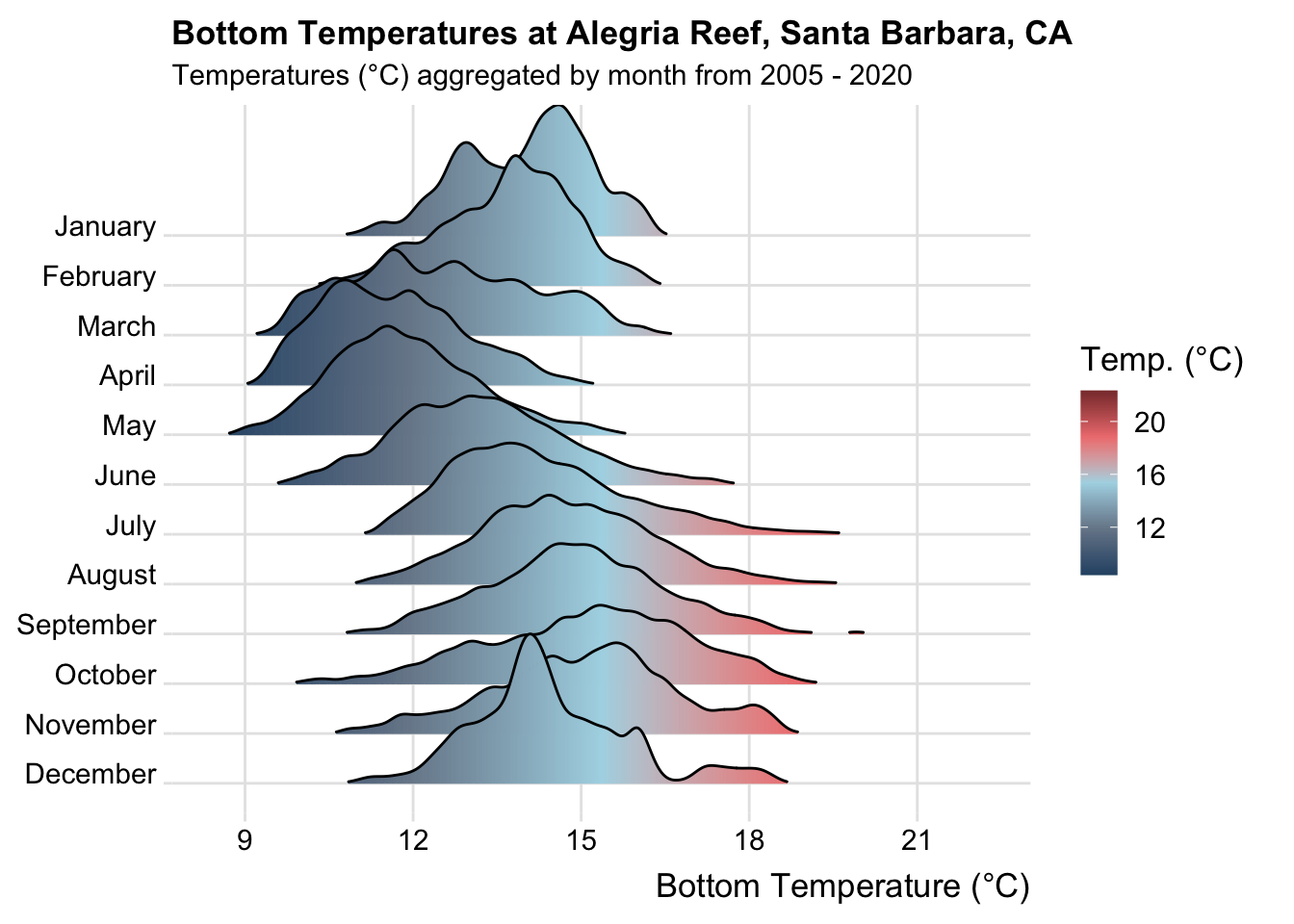

If we were to continue with this workflow (which is absolutely a valid way that gets the job done!), we would need to repeat the above code two more times (for both the mohawk and carpinteria data frames) – this gets lengthy rather quickly, requires lots of copying/pasting, and is prone to errors (e.g. forgetting to update a data frame name, typos, etc.). If you’d like to check out the code for the mohawk and carpinteria data sets, unfold the code chunk below:

Code

#..........................Mohawk Reef...........................

# clean ----
mohawk_clean <- mohawk |> 
  select(year, month, day, decimal_time, Temp_top, Temp_mid, Temp_bot) |>
  filter(year %in% c(2005:2020)) |> 
  mutate(site = rep("Mohawk Reef")) |> 
  unite(col = date, year, month, day, sep = "-", remove = FALSE) |> 
  mutate(time = times(decimal_time)) |> 
  unite(col = date_time, date, time, sep = " ", remove = TRUE) |> 
  mutate(date_time = as.POSIXct(date_time, "%Y-%m-%d %H:%M:%S", tz = "GMT"),
         year = as.factor(year),
         month = as.factor(month),
         day = as.numeric(day)) |>
  mutate(month_name = as.factor(month.name[month])) |>
  replace_with_na(replace = list(Temp_bot = 9999, Temp_top = 9999, Temp_mid = 9999)) |> 
  select(site, date_time, year, month, day, month_name, Temp_bot, Temp_mid, Temp_top)

# plot ----
mohawk_plot <- mohawk_clean |> 
  group_by(month_name) |> 
  ggplot(aes(x = Temp_bot, y = month_name, fill = after_stat(x))) +
  geom_density_ridges_gradient(rel_min_height = 0.01, scale = 3) + 
  scale_x_continuous(breaks = c(9, 12, 15, 18, 21)) +
  scale_y_discrete(limits = rev(month.name)) + 
  scale_fill_gradientn(colors = c("#2C5374","#778798", "#ADD8E6", "#EF8080", "#8B3A3A"), name = "Temp. (°C)") +
  labs(x = "Bottom Temperature (°C)",
       title = "Bottom Temperatures at Mohawk Reef, Santa Barbara, CA",
       subtitle = "Temperatures (°C) aggregated by month from 2005 - 2020") +
  ggridges::theme_ridges(font_size = 13, grid = TRUE) +
  theme(
    axis.title.y = element_blank()
  )

mohawk_plot
#........................Carpinteria Reef........................

# clean ----
carpinteria_clean <- carpinteria |> 
  select(year, month, day, decimal_time, Temp_top, Temp_mid, Temp_bot) |>
  filter(year %in% c(2005:2020)) |> 
  mutate(site = rep("Carpinteria Reef")) |> 
  unite(col = date, year, month, day, sep = "-", remove = FALSE) |> 
  mutate(time = times(decimal_time)) |> 
  unite(col = date_time, date, time, sep = " ", remove = TRUE) |> 
  mutate(date_time = as.POSIXct(date_time, "%Y-%m-%d %H:%M:%S", tz = "GMT"),
         year = as.factor(year),
         month = as.factor(month),
         day = as.numeric(day)) |>
  mutate(month_name = as.factor(month.name[month])) |>
  replace_with_na(replace = list(Temp_bot = 9999, Temp_top = 9999, Temp_mid = 9999)) |> 
  select(site, date_time, year, month, day, month_name, Temp_bot, Temp_mid, Temp_top)

# plot ----
carpinteria_plot <- carpinteria_clean |> 
  group_by(month_name) |> 
  ggplot(aes(x = Temp_bot, y = month_name, fill = after_stat(x))) +
  geom_density_ridges_gradient(rel_min_height = 0.01, scale = 3) + 
  scale_x_continuous(breaks = c(9, 12, 15, 18, 21)) +
  scale_y_discrete(limits = rev(month.name)) + 
  scale_fill_gradientn(colors = c("#2C5374","#778798", "#ADD8E6", "#EF8080", "#8B3A3A"), name = "Temp. (°C)") +
  labs(x = "Bottom Temperature (°C)",
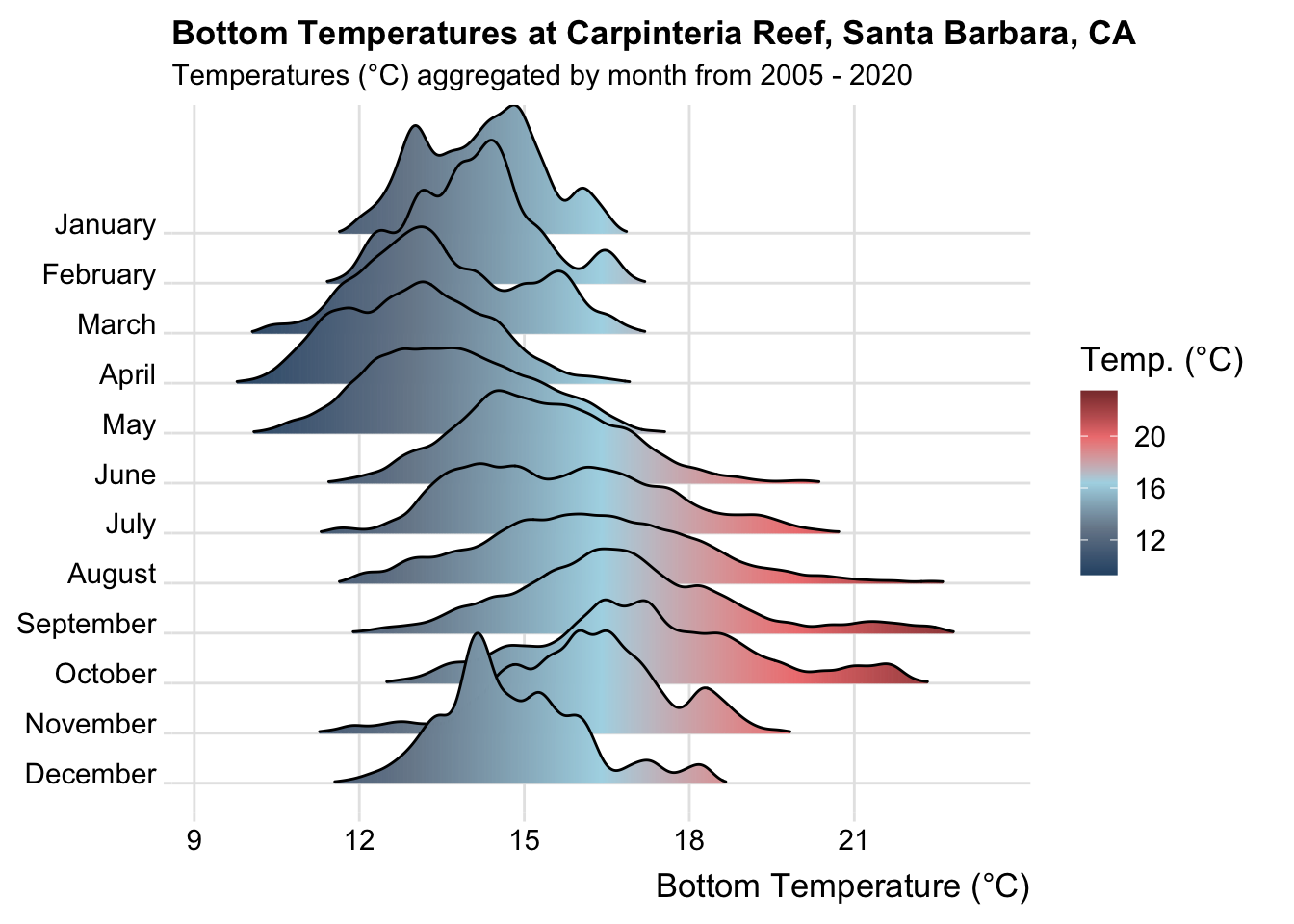
       title = "Bottom Temperatures at Carpinteria Reef, Santa Barbara, CA",
       subtitle = "Temperatures (°C) aggregated by month from 2005 - 2020") +
  ggridges::theme_ridges(font_size = 13, grid = TRUE) +
  theme(
    axis.title.y = element_blank()
  )

carpinteria_plot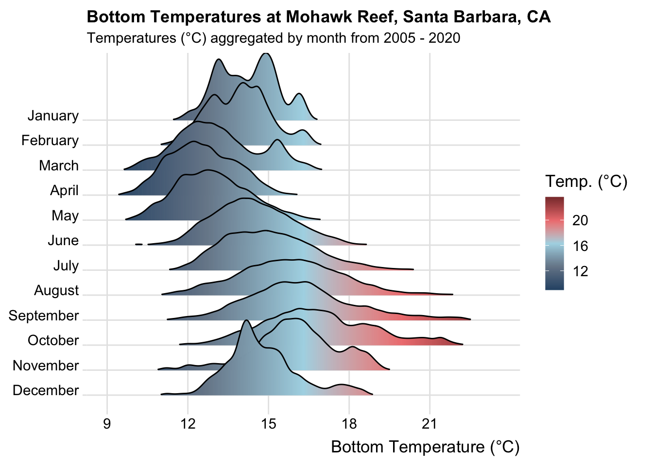

Stage 2: Write functions to clean & plot your data

Though there isn’t anything inherently wrong with copying/pasting large chunks of code, it’s a better practice to turn repeated code into functions. In Stage 2, we’ll turn our cleaning and plotting pipelines into functions that can be called on any of our similarly-structured data sets.

Where do I write/save my functions?

While there’s no hard and fast rule, I tend to create a subdirectory within my project (e.g. named /R, /utils, etc.) to house all my function scripts. I prefer to create a separate .R script for each of my functions, and name each file the same as the function itself (e.g. if I’m writing a function called do_fun_thing(), I’d save it to a script called do_fun_thing.R).

You can then source your function files into whatever script (or .rmd/.qmd file) where you call that function (e.g. source("utils/do_fun_thing.R").

Note: You cannot source() a .rmd or .qmd file into another file/script, therefore it’s important to save functions to a .R file.

Here, let’s create the following:

a /utils folder to store our functions scripts
a clean_ocean_temps.R file (saved to /utils), where we’ll write a function to clean our data
a plot_ocean_temps.R file (saved to /utils), where we’ll write a function to plot our data
a functions_pipeline.R file (saved to the root directory), where we’ll use our functions to clean and plot our data – you can also read-in your data files here, just as we did in Stage 1, part ii

i. Write a function to clean data sets

It’s helpful to first identify which parts of the cleaning code need to be generalized/made “flexible” so that any of our three data frames can be passed to it for cleaning. For us, that’s the name of the raw data frame and the site name character string that’s repeated for the length of the added site column (see annotation notes below the rendered code):

1alegria_clean <- alegria |>
  select(year, month, day, decimal_time, Temp_top, Temp_mid, Temp_bot) |>
  filter(year %in% c(2005:2020)) |> 
2  mutate(site = rep("Alegria Reef")) |>
  unite(col = date, year, month, day, sep = "-", remove = FALSE) |> 
  mutate(time = times(decimal_time)) |> 
  unite(col = date_time, date, time, sep = " ", remove = TRUE) |> 
  mutate(date_time = as.POSIXct(date_time, "%Y-%m-%d %H:%M:%S", tz = "GMT"),
         year = as.factor(year),
         month = as.factor(month),
         day = as.numeric(day)) |>
  mutate(month_name = as.factor(month.name[month])) |>
  replace_with_na(replace = list(Temp_bot = 9999, Temp_top = 9999, Temp_mid = 9999)) |> 
  select(site, date_time, year, month, day, month_name, Temp_bot, Temp_mid, Temp_top)

1: the name of the raw data frame (here, alegria) needs to be generalized
2: the site name character string that’s repeated for the length of the added site column (here, “Alegria Reef”) needs to be generalized

Now we can start to build out our function. We’ll start by creating a super basic function, then build in more complexity. I encourage you to test out your function after each version to ensure that it works as you intend it to.

Version 1:

The primary goal of clean_ocean_temps() v1 is to get a basic data cleaning function working.

To start, let’s create the skeleton of our function, which we’ll call clean_ocean_temps():

clean_ocean_temps <- function(){
  
}

Now, let’s copy and paste our cleaning code for Alegria Reef data (from Stage 1, above) into the body of the function (i.e. within the curly brackets, {}).

clean_ocean_temps <- function(){
 
  alegria_clean <- alegria |> 
    select(year, month, day, decimal_time, Temp_top, Temp_mid, Temp_bot) |>
    filter(year %in% c(2005:2020)) |> 
    mutate(site = rep("Alegria Reef")) |> 
    unite(col = date, year, month, day, sep = "-", remove = FALSE) |> 
    mutate(time = times(decimal_time)) |> 
    unite(col = date_time, date, time, sep = " ", remove = TRUE) |> 
    mutate(date_time = as.POSIXct(date_time, "%Y-%m-%d %H:%M:%S", tz = "GMT"),
          year = as.factor(year),
          month = as.factor(month),
          day = as.numeric(day)) |>
    mutate(month_name = as.factor(month.name[month])) |>
    replace_with_na(replace = list(Temp_bot = 9999, Temp_top = 9999, Temp_mid = 9999)) |> 
    select(site, date_time, year, month, day, month_name, Temp_bot, Temp_mid, Temp_top)
  
}

Next, we want the ability to provide our function with any three of our data sets for processing. To do so, we’ll make the following updates:

1clean_ocean_temps <- function(raw_data){
  
  # clean data ----
2  temps_clean <- raw_data |>
    select(year, month, day, decimal_time, Temp_top, Temp_mid, Temp_bot) |>
    filter(year %in% c(2005:2020)) |> 
4    mutate(site = rep("_____")) |>
    unite(col = date, year, month, day, sep = "-", remove = FALSE) |> 
    mutate(time = times(decimal_time)) |> 
    unite(col = date_time, date, time, sep = " ", remove = TRUE) |> 
    mutate(date_time = as.POSIXct(date_time, "%Y-%m-%d %H:%M:%S", tz = "GMT"),
          year = as.factor(year),
          month = as.factor(month),
          day = as.numeric(day)) |>
    mutate(month_name = as.factor(month.name[month])) |>
    replace_with_na(replace = list(Temp_bot = 9999, Temp_top = 9999, Temp_mid = 9999)) |> 
    select(site, date_time, year, month, day, month_name, Temp_bot, Temp_mid, Temp_top)
  
  # return cleaned df ----
3  return(temps_clean)
}

1: create an input (aka argument) called raw_data inside function() (NOTE: you can name your argument however you’d like, but preferably something short and descriptive)
2: replace our hard-coded data frame name (e.g. alegria in the previous code chunk) in our cleaning pipeline with raw_data
3: update the name of the object we save our clean data to (currently alegria_clean) to something a bit more generalized, like temps_clean, and return() our clean data frame object at the end of the function
4: recall that part of our cleaning pipeline includes adding a column called site, with repeating values that are the site name; for now, let’s just add some placeholder text (“_____”) and we’ll figure out how to make that text match up with the data in the next versions of our function

What is return() and when is it necessary?

Oftentimes, we want a function to do some processing on whatever we provide it and then give us back the result. We use the return() function to do this in R.

R automatically returns the the last output of a function – here, it isn’t necessary to return(temps_clean) since the temps_clean data frame is the last output of our clean_ocean_temps() function.

An explicit return() is used to return a value immediately from a function. If it is not the last statement of a function, return() will prematurely end the function – for example, if x = 2, the string, "Positive" will be returned (and the remaining if else statement will not be executed):

check_number <- function(x) {
  if (x > 0) {
    return("Positive")
  }
  else if (x < 0) {
    return("Negative")
  }
  else {
    return("Zero")
  }
}

I tend to include an explicit return() at the end of my functions because I think it makes it easier to read/understand the code, but check out this interesting dialogue on whether this is best practice or not.

Lastly, let’s make sure our function works. You can take a few approaches to trying out your work:

test in the console: I do this a lot! It’s fast and allows you to test out different things if you encounter any sticking points. You’ll see me doing that while teaching
write and run your functions_pipeline.R script: Begin writing your analysis script (here, that’s functions_pipeline.R) – below is one way you might consider setting up your script

Regardless, make sure to always rerun/re-source your function after making changes so that an updated version gets saved to your global environment!

# functions_pipeline.R #

#..........................load packages......................... 
1library(readr)
library(dplyr)
library(tidyr)
library(chron)
library(naniar)

#........................source functions........................ 
2source("utils/clean_ocean_temps.R")

#..........................import data........................... 
3alegria <- read_csv(here::here("data", "raw_data", "alegria_mooring_ale_20210617.csv"))
mohawk <- read_csv(here::here("data", "raw_data", "mohawk_mooring_mko_20220330.csv"))
carpinteria <- read_csv(here::here("data", "raw_data", "carpinteria_mooring_car_20220330.csv"))

#...........................clean data........................... 
4alegria_clean <- clean_ocean_temps(raw_data = alegria)
mohawk_clean <- clean_ocean_temps(raw_data = mohawk)
carpinteria_clean <- clean_ocean_temps(raw_data = carpinteria)

1: make sure any packages that your function relies on are installed/imported ¹
2: source your function into your script
3: read in your data
4: use your clean_ocean_temps() function to process your raw data

Version 2:

The primary goal of clean_ocean_temps() v2 is to create a site column that contains the correct site name.

There are lots of creative ways to go about forming the site name that will get added as a repeating value to the site column, but the easiest and most explicit is likely adding a second function argument that takes the site name as a character string (e.g. site_name = "alegria")

Let’s add that to our function:

1clean_ocean_temps <- function(raw_data, site_name){

  # format `site_name` ----
2  site_name_formatted <- paste(str_to_title(site_name), "Reef")
    
  # clean data ----
  temps_clean <- raw_data |> 
    select(year, month, day, decimal_time, Temp_top, Temp_mid, Temp_bot) |>
    filter(year %in% c(2005:2020)) |> 
3    mutate(site = rep(site_name_formatted)) |>
    unite(col = date, year, month, day, sep = "-", remove = FALSE) |> 
    mutate(time = times(decimal_time)) |> 
    unite(col = date_time, date, time, sep = " ", remove = TRUE) |> 
    mutate(date_time = as.POSIXct(date_time, "%Y-%m-%d %H:%M:%S", tz = "GMT"),
          year = as.factor(year),
          month = as.factor(month),
          day = as.numeric(day)) |>
    mutate(month_name = as.factor(month.name[month])) |>
    replace_with_na(replace = list(Temp_bot = 9999, Temp_top = 9999, Temp_mid = 9999)) |> 
    select(site, date_time, year, month, day, month_name, Temp_bot, Temp_mid, Temp_top)
  
  # return cleaned df ----
  return(temps_clean) 
  
}

1: add a second argument called site_name (or something intuitive)
2: we might specify in our function documentation that site_name takes the standard site name (as used by SBC LTER) as a character string, but what happens if a users uses different character casing than expected (e.g. "alegria", "MOHAWK", "Carpinteria")? We can use a combination of paste() and the {stringr} package to format that value as we’d like it to appear in our site column – here, that’s converting it to Title Case and pasting "Reef" at the end (e.g. "alegria" will become "Alegria Reef") ; I referenced this resource)
3: substitute our formatted character string, site_name_formatted, in for the hard-coded site name in mutate(site = rep("___ Reef"))

Rerun the updated function and try using it to make sure the appropriate site name is added to the site_name column for each of the data sets:

# functions_pipeline.R #

#..........................load packages.........................  
library(readr)
library(dplyr) 
library(tidyr)
1library(stringr)
library(chron)
library(naniar)

#........................source functions........................  
source("utils/clean_ocean_temps.R") 

#..........................import data...........................  
alegria <- read_csv(here::here("data", "raw_data", "alegria_mooring_ale_20210617.csv"))
mohawk <- read_csv(here::here("data", "raw_data", "mohawk_mooring_mko_20220330.csv"))
carpinteria <- read_csv(here::here("data", "raw_data", "carpinteria_mooring_car_20220330.csv"))

#...........................clean data...........................  
2alegria_clean <- clean_ocean_temps(raw_data = alegria, site_name = "alegria")
mohawk_clean <- clean_ocean_temps(raw_data = mohawk, site_name = "MOHAWK")
carpinteria_clean <- clean_ocean_temps(raw_data = carpinteria, site_name = "Carpinteria")

1: remember to import the {stringr} package, since we’ll be using stringr::replace_with_na() within our function
2: add in the site_name argument – here, we demonstrate that how our function handles formatting, regardless of character case

Version 3:

The primary goal of `clean_ocean_temps() v3 is to provide a way for users to select which temperature measurements (Temp_top, Temp_mid, Temp_bot) to include in the cleaned data frame.

Our function works perfectly fine as-is, but let’s say we don’t always want all three temperature measurements (surface temperature (Temp_top), mid-column temperature (Temp_mid), and bottom temperature (Temp_top)) included in our cleaned data. We can build flexibility into our function by adding an argument that allows the user to select exactly which of the three temperature measurements to include in the resulting cleaned data frame. To do this, we’ll make the following changes:

1clean_ocean_temps <- function(raw_data, site_name, include_temps = c("Temp_top", "Temp_mid", "Temp_bot")){
  
  # format `site_name` ----
  site_name_formatted <- paste(str_to_title(site_name), "Reef")
  
  # columns to select ---- 
2  always_selected_cols <- c("year", "month", "day", "decimal_time")
3  all_cols <- append(always_selected_cols, include_temps)
  
  # clean data ----
  temps_clean <- raw_data |> 
4    select(all_of(all_cols)) |>
    filter(year %in% c(2005:2020)) |> 
    mutate(site = rep(site_name_formatted)) |> 
    unite(col = date, year, month, day, sep = "-", remove = FALSE) |> 
    mutate(time = times(decimal_time)) |> 
    unite(col = date_time, date, time, sep = " ", remove = TRUE) |> 
    mutate(date_time = as.POSIXct(date_time, "%Y-%m-%d %H:%M:%S", tz = "GMT"),
           year = as.factor(year),
           month = as.factor(month),
           day = as.numeric(day)) |>
    mutate(month_name = as.factor(month.name[month])) |>
    replace_with_na(replace = list(Temp_bot = 9999, Temp_top = 9999, Temp_mid = 9999)) |> 
5    select(any_of(c("site", "date_time", "year", "month", "day", "month_name", "Temp_bot", "Temp_mid", "Temp_top")))
  
  # return cleaned df ----
  return(temps_clean) 
}

1: add a third argument called include_temps, which defaults to including all three temperature variables (Temp_top, Temp_mid, Temp_bot)
2: create a vector of variable names that should always be selected
3: combine the “always selected” variables with the user-selected variables as specified using the include_temps argument
4: select columns based on variables names in our all_cols vector using select(all_of()) ( I first got an error message ² when attempting to select(all_cols), since an external vector alone can’t be used to make selections; I then referenced this resource)
5: make our last select call ³, which is used to reorder columns, flexible enough to reorder temperature variables which may or may not be present using select(any_of()) ( I again referenced this resource)

Rerun the updated function and try out our new inlcude_temps argument:

# functions_pipeline.R #

#..........................load packages.........................  
library(readr)
library(dplyr) 
library(tidyr)
library(stringr) 
library(chron)
library(naniar)

#........................source functions........................ 
source("utils/clean_ocean_temps.R") 

#..........................import data...........................  
alegria <- read_csv(here::here("data", "raw_data", "alegria_mooring_ale_20210617.csv"))
mohawk <- read_csv(here::here("data", "raw_data", "mohawk_mooring_mko_20220330.csv"))
carpinteria <- read_csv(here::here("data", "raw_data", "carpinteria_mooring_car_20220330.csv"))

#...........................clean data........................... 
1alegria_clean <- clean_ocean_temps(raw_data = alegria, site_name = "alegria", include_temps = c("Temp_bot")) # includes only `Temp_bot`
mohawk_clean <- clean_ocean_temps(raw_data = mohawk, site_name = "MOHAWK") # includes all three temp cols (`Temp_top`, `Temp_mid`, `Temp_bot`) by default
carpinteria_clean <- clean_ocean_temps(raw_data = carpinteria, site_name = "Carpinteria", include_temps = c("Temp_mid", "Temp_bot")) # includes only `Temp_mid` & `Temp_bot`

1: try using our new include_temps argument to return a cleaned data frame with a subset of the temperature measurement variables

Note: naniar::replace_with_na() may throw a warning message

However this will not halt execution – if one or more of the temperature variables are missing (e.g. if we specify include_temps = c("Temp_bot"), you will get a warning that says, Missing from data: Temp_top, Temp_mid).

Version 4:

The primary goal of clean_ocean_temps() v4 is to build in checks to ensure that the data provided to the function is compatible with the cleaning pipeline (i.e. ensure that the correct columns are present.

To wrap things up, we might consider adding an if else statement that checks to ensure that the data provided is suitable for our cleaning pipeline:

clean_ocean_temps <- function(raw_data, site_name, include_temps = c("Temp_top", "Temp_mid", "Temp_bot")){ 
  
  # if data contains these colnames, clean the script ----
1  if(all(c("year", "month", "day", "decimal_time", "Temp_bot", "Temp_top", "Temp_mid") %in% colnames(raw_data))) {
    
    message("Cleaning data...")
    
    # format `site_name` ----
    site_name_formatted <- paste(str_to_title(site_name), "Reef")
    
    # columns to select ----
    standard_cols <- c("year", "month", "day", "decimal_time") 
    all_cols <- append(standard_cols, include_temps) 
    
    # clean data ----
    temps_clean <- raw_data |> 
      select(all_of(all_cols)) |> 
      filter(year %in% c(2005:2020)) |> 
      mutate(site = rep(site_name_formatted)) |> 
      unite(col = date, year, month, day, sep = "-", remove = FALSE) |> 
      mutate(time = times(decimal_time)) |> 
      unite(col = date_time, date, time, sep = " ", remove = TRUE) |> 
      mutate(date_time = as.POSIXct(date_time, "%Y-%m-%d %H:%M:%S", tz = "GMT"),
             year = as.factor(year),
             month = as.factor(month),
             day = as.numeric(day)) |>
      mutate(month_name = as.factor(month.name[month])) |>
      replace_with_na(replace = list(Temp_bot = 9999, Temp_top = 9999, Temp_mid = 9999)) |> 
      select(any_of(c("site", "date_time", "year", "month", "day", "month_name", "Temp_bot", "Temp_mid", "Temp_top")))
    
    # return cleaned df ----
    return(temps_clean)
    
2  } else {
    
    stop("The data frame provided does not include the necessary columns. Double check your data!")
    
  }
  
}

1: add an if else statement that checks whether the necessary columns are present in the raw data – if yes, proceed with data cleaning
2: if no, throw an error message

Let’s rerun our function and try it out one last time:

# functions_pipeline.R #

#..........................load packages.........................  
library(readr)
library(dplyr) 
library(tidyr)
library(stringr) 
library(chron)
library(naniar)

#........................source functions........................ 
source("utils/clean_ocean_temps.R") 

#..........................import data...........................  
alegria <- read_csv(here::here("data", "raw_data", "alegria_mooring_ale_20210617.csv"))
mohawk <- read_csv(here::here("data", "raw_data", "mohawk_mooring_mko_20220330.csv"))
carpinteria <- read_csv(here::here("data", "raw_data", "carpinteria_mooring_car_20220330.csv"))

#...........................clean data...........................  
1alegria_clean <- clean_ocean_temps(raw_data = alegria, site_name = "alegria", include_temps = c("Temp_bot"))
mohawk_clean <- clean_ocean_temps(raw_data = mohawk, site_name = "MOHAWK")
carpinteria_clean <- clean_ocean_temps(raw_data = carpinteria, site_name = "Carpinteria", include_temps = c("Temp_mid", "Temp_bot"))
2penguins_clean <- clean_ocean_temps(raw_data = palmerpenguins::penguins)

1: these three should work as intended
2: this one should throw an error!

ii: Write a function to plot data sets

Similar to what we did for our cleaning code, let’s first identify which parts of the plotting code need to be generalized/made “flexible” so that any of our three cleaned data frames can be passed to it for plotting. For us, that’s the name of the clean data frame and the site name that appears in the plot title (see annotation notes below the rendered code):

1alegria_plot <- alegria_clean |>
  group_by(month_name) |> 
  ggplot(aes(x = Temp_bot, y = month_name, fill = after_stat(x))) +
  geom_density_ridges_gradient(rel_min_height = 0.01, scale = 3) + 
  scale_x_continuous(breaks = c(9, 12, 15, 18, 21)) +
  scale_y_discrete(limits = rev(month.name)) + 
  scale_fill_gradientn(colors = c("#2C5374","#778798", "#ADD8E6", "#EF8080", "#8B3A3A"), name = "Temp. (°C)") +
  labs(x = "Bottom Temperature (°C)",
2       title = "Bottom Temperatures at Alegria Reef, Santa Barbara, CA",
       subtitle = "Temperatures (°C) aggregated by month from 2005 - 2020") +
  ggridges::theme_ridges(font_size = 13, grid = TRUE) +
  theme(
    axis.title.y = element_blank()
  )

alegria_plot

1: the name of the clean data frame needs to be generalized
2: the site name that appears in the plot title needs to be generalized

Version 1:

The primary goal of plot_ocean_temps v1 is to get a basic plotting function working.

Now we can begin to building our function. Let’s again start by creating the skeleton of our function, which we’ll call plot_ocean_temps():

plot_ocean_temps <- function(){
  
}

…then copy and paste our plotting code for the clean Alegria Reef data into the body of the function (i.e. within the curly brackets, {}).

plot_ocean_temps <- function() {

  alegria_plot <- alegria_clean |> 
    group_by(month_name) |> 
    ggplot(aes(x = Temp_bot, y = month_name, fill = after_stat(x))) +
    geom_density_ridges_gradient(rel_min_height = 0.01, scale = 3) + 
    scale_x_continuous(breaks = c(9, 12, 15, 18, 21)) +
    scale_y_discrete(limits = rev(month.name)) + 
    scale_fill_gradientn(colors = c("#2C5374","#778798", "#ADD8E6", "#EF8080", "#8B3A3A"), name = "Temp. (°C)") +
    labs(x = "Bottom Temperature (°C)",
         title = "Bottom Temperatures at Alegria Reef, Santa Barbara, CA",
         subtitle = "Temperatures (°C) aggregated by month from 2005 - 2020") +
    ggridges::theme_ridges(font_size = 13, grid = TRUE) +
    theme(
      axis.title.y = element_blank()
    )
  
}

Just like in clean_ocean_temps(), we want the ability to provide our function with any three of our cleaned data sets for plotting. To do this, we’ll make the following modifications:

1plot_ocean_temps <- function(clean_data) {

  # plot data ----
2  temps_plot <- clean_data |>
    group_by(month_name) |> 
    ggplot(aes(x = Temp_bot, y = month_name, fill = after_stat(x))) +
    geom_density_ridges_gradient(rel_min_height = 0.01, scale = 3) + 
    scale_x_continuous(breaks = c(9, 12, 15, 18, 21)) +
    scale_y_discrete(limits = rev(month.name)) + 
    scale_fill_gradientn(colors = c("#2C5374","#778798", "#ADD8E6", "#EF8080", "#8B3A3A"), name = "Temp. (°C)") +
    labs(x = "Bottom Temperature (°C)",
4         title = "Bottom Temperatures at _____, Santa Barbara, CA",
         subtitle = "Temperatures (°C) aggregated by month from 2005 - 2020") +
    ggridges::theme_ridges(font_size = 13, grid = TRUE) +
    theme(
      axis.title.y = element_blank()
    )
  
  # return plot ----
3  return(temps_plot)
  
}

1: create an input (aka argument) called clean_data inside function() (NOTE: you can name your argument however you’d like, but preferably something short and descriptive)
2: replace our hard-coded data frame name (e.g. alegria_clean in the code above) in our plotting pipeline with our new argument, clean_data
3: update the name of the object we save our plot output to (currently alegria_plot) to something a bit more generalized, like temps_plot and return() our plot object at the end
4: and add some placeholder text (“_____”) in the title field where the site name should be – we’ll make this flexible in our next version

Now let’s make sure our function works. Run the function so that it’s saved to our global environment, then use it to try plotting our cleaned data sets:

# functions_pipeline.R #

#..........................load packages.........................  
library(readr)
library(dplyr) 
library(tidyr)
library(stringr) 
library(chron)
library(naniar)
1library(ggplot2)
library(ggridges)

#........................source functions........................  
source("utils/clean_ocean_temps.R") 
source("utils/plot_ocean_temps.R")

#..........................import data...........................  
alegria <- read_csv(here::here("data", "raw_data", "alegria_mooring_ale_20210617.csv"))
mohawk <- read_csv(here::here("data", "raw_data", "mohawk_mooring_mko_20220330.csv"))
carpinteria <- read_csv(here::here("data", "raw_data", "carpinteria_mooring_car_20220330.csv"))

#...........................clean data...........................  
alegria_clean <- clean_ocean_temps(raw_data = alegria, site_name = "alegria", include_temps = c("Temp_bot")) 
mohawk_clean <- clean_ocean_temps(raw_data = mohawk, site_name = "MOHAWK") 
carpinteria_clean <- clean_ocean_temps(raw_data = carpinteria, site_name = "Carpinteria", include_temps = c("Temp_mid", "Temp_bot")) 

#............................plot data...........................
2alegria_plot <- plot_ocean_temps(clean_data = alegria_clean)
mohawk_plot <- plot_ocean_temps(clean_data = mohawk_clean)
carpinteria_plot <- plot_ocean_temps(clean_data = carpinteria_clean)

1: make sure any additional packages that our plot_ocean_temps() function relies on are installed/imported
2: Reminder: plot_ocean_temps() is written so that it plots bottom temperatures (Temp_bot), so make sure that your cleaned data sets have this variable present (i.e. make sure that include_temps is set to it’s default or that Temp_bot is explicitly included)

Version 2:

The primary goal of plot_ocean_temps() v2 is to to create a plot title that contains the correct side name.

In this next version, let’s figure out how to update the plot title so that the appropriate site name appears each time a different data set is plotted. Luckily for us, we’ve already added a site column to our *_clean data, which contains the site name as a character string. We can extract this site name by adding the following:

plot_ocean_temps <- function(clean_data) { 

  # get site name for plot title ----
1  site_name <- unique(clean_data$site)
  
  # plot data ----
  temp_plot <- clean_data |> 
    group_by(month_name) |> 
    ggplot(aes(x = Temp_bot, y = month_name, fill = after_stat(x))) +
    ggridges::geom_density_ridges_gradient(rel_min_height = 0.01, scale = 3) + 
    scale_x_continuous(breaks = c(9, 12, 15, 18, 21)) +
    scale_y_discrete(limits = rev(month.name)) + 
    scale_fill_gradientn(colors = c("#2C5374","#778798", "#ADD8E6", "#EF8080", "#8B3A3A"), name = "Temp. (°C)") +
    labs(x = "Bottom Temperature (°C)",
2         title = paste("Bottom Temperatures at ",  site_name, ", Santa Barbara, CA", sep = ""),
         subtitle = "Temperatures (°C) aggregated by month from 2005 - 2022") +
    ggridges::theme_ridges(font_size = 13, grid = TRUE) +
    theme(
      axis.title.y = element_blank()
    )
  
  # return plot ----
  return(temp_plot)
}

1: use the unique() function to get the site name for a given data set; recall that we should only have 1 unique site name per data set
2: use the paste() function to construct a title using our extracted site name

Rerun and try out your function again to make sure it works as expected:

# functions_pipeline.R #

#..........................load packages.........................  
library(readr)
library(dplyr) 
library(tidyr)
library(stringr) 
library(chron)
library(naniar)
library(ggplot2)
library(ggridges) 

#........................source functions........................  
source("utils/clean_ocean_temps.R") 
1source("utils/plot_ocean_temps.R")

#..........................import data...........................  
alegria <- read_csv(here::here("data", "raw_data", "alegria_mooring_ale_20210617.csv"))
mohawk <- read_csv(here::here("data", "raw_data", "mohawk_mooring_mko_20220330.csv"))
carpinteria <- read_csv(here::here("data", "raw_data", "carpinteria_mooring_car_20220330.csv"))

#...........................clean data...........................  
alegria_clean <- clean_ocean_temps(raw_data = alegria, site_name = "alegria", include_temps = c("Temp_bot")) 
mohawk_clean <- clean_ocean_temps(raw_data = mohawk, site_name = "MOHAWK") 
carpinteria_clean <- clean_ocean_temps(raw_data = carpinteria, site_name = "Carpinteria", include_temps = c("Temp_mid", "Temp_bot")) 

#............................plot data...........................
alegria_plot <- plot_ocean_temps(clean_data = alegria_clean) 
mohawk_plot <- plot_ocean_temps(clean_data = mohawk_clean) 
carpinteria_plot <- plot_ocean_temps(clean_data = carpinteria_clean)

1: remember to re-load your function after you make changes!

iii: Putting it all together

Okay, now let’s bring all these pieces together! Our revised scripts might look something like this:

#..........................load packages......................... 
library(readr)
library(dplyr) 
library(tidyr)
library(stringr) 
library(chron)
library(naniar)
library(ggplot2)
library(ggridges) 

#........................source functions........................  
source("utils/clean_ocean_temps.R") 
source("utils/plot_ocean_temps.R") 

#..........................import data...........................  
alegria <- read_csv(here::here("data", "raw_data", "alegria_mooring_ale_20210617.csv"))
mohawk <- read_csv(here::here("data", "raw_data", "mohawk_mooring_mko_20220330.csv"))
carpinteria <- read_csv(here::here("data", "raw_data", "carpinteria_mooring_car_20220330.csv"))

#...........................clean data...........................  
alegria_clean <- clean_ocean_temps(raw_data = alegria, site_name = "alegria", include_temps = c("Temp_bot")) 
mohawk_clean <- clean_ocean_temps(raw_data = mohawk, site_name = "MOHAWK") 
carpinteria_clean <- clean_ocean_temps(raw_data = carpinteria, site_name = "Carpinteria", include_temps = c("Temp_mid", "Temp_bot"))

#............................plot data...........................
alegria_plot <- plot_ocean_temps(clean_data = alegria_clean) 
mohawk_plot <- plot_ocean_temps(clean_data = mohawk_clean) 
carpinteria_plot <- plot_ocean_temps(clean_data = carpinteria_clean)

Use a roxygen skeleton to document your function

Even if you don’t plan to publish your function as part of a package, documenting your work is still a critical part of reproducibility and usability. This may be done in more informal ways, such as code annotations and text explanations in RMarkdown documents, for example. You may also consider more formal documentation – the {roxygen2} package helps to make that process easier. Click anywhere inside your function, then choose Code > Insert Roxygen Skeleton to get started.

#' Process CTD/ADCP temperature data
#'
#' @param raw_data data frame of CTD/ADCP data collected at SBC LTER site moorings; search for data on the EDI Data Portal (http://portal.edirepository.org:80/nis/simpleSearch?defType=edismax&q=SBC+LTER%5C%3A+Ocean%5C%3A+Currents+and+Biogeochemistry%5C%3A+Moored+CTD+and+ADCP+data&fq=-scope:ecotrends&fq=-scope:lter-landsat*&fl=id,packageid,title,author,organization,pubdate,coordinates&debug=false)
#' @param site_name Santa Barbara Coastal LTER site name as a character string
#' @param include_temps vector of character strings that includes one or more of the following variable names: Temp_top, Temp_mid, Temp_top
#'
#' @return a data frame
#' @export
#'
#' @examples
#' my_clean_df <- clean_ocean_temps(raw_data = my_raw_df, include_temps = c("Temp_bot"))
clean_ocean_temps <- function(raw_data, site_name, include_temps = c("Temp_top", "Temp_mid", "Temp_bot")){ 
  
  # if data contains these colnames, clean the script ----
  if(all(c("year", "month", "day", "decimal_time", "Temp_bot", "Temp_top", "Temp_mid") %in% colnames(raw_data))) { 
    
    message("Cleaning data...") 
    
    # format site name ----
    site_name_formatted <- paste(str_to_title(site_name), "Reef")
    
    # columns to select ----
    standard_cols <- c("year", "month", "day", "decimal_time") 
    all_cols <- append(standard_cols, include_temps) 
    
    # clean data ----
    temps_clean <- raw_data |> 
      select(all_of(all_cols)) |> 
      filter(year %in% c(2005:2020)) |> 
      mutate(site = rep(site_name_formatted)) |> 
      unite(col = date, year, month, day, sep = "-", remove = FALSE) |> 
      mutate(time = times(decimal_time)) |> 
      unite(col = date_time, date, time, sep = " ", remove = TRUE) |> 
      mutate(date_time = as.POSIXct(date_time, "%Y-%m-%d %H:%M:%S", tz = "GMT"),
             year = as.factor(year),
             month = as.factor(month),
             day = as.numeric(day)) |>
      mutate(month_name = as.factor(month.name[month])) |>
      replace_with_na(replace = list(Temp_bot = 9999, Temp_top = 9999, Temp_mid = 9999)) |> 
      select(any_of(c("site", "date_time", "year", "month", "day", "month_name", "Temp_bot", "Temp_mid", "Temp_top")))
    
    # return cleaned df ----
    return(temps_clean) 
    
  } else { 
    
    stop("The data frame provided does not include the necessary columns. Double check your data!") 
    
  }
  
}

Use a roxygen skeleton to document your function

#' Create ridge line plot of CTD/ADCP bottom temperature data
#'
#' @param clean_data a data frame that has been pre-processed using clean_ocean_temp()
#'
#' @return a plot object
#' @export
#'
#' @examples
#' my_plot <- plot_ocean_temps(clean_data = my_clean_df)
plot_ocean_temps <- function(clean_data) { 
  
  # get site name for plot title ----
  site_name <- unique(clean_data$site)
  
  # plot data ----
  temp_plot <- clean_data |> 
    group_by(month_name) |> 
    ggplot(aes(x = Temp_bot, y = month_name, fill = after_stat(x))) +
    ggridges::geom_density_ridges_gradient(rel_min_height = 0.01, scale = 3) + 
    scale_x_continuous(breaks = c(9, 12, 15, 18, 21)) +
    scale_y_discrete(limits = rev(month.name)) + 
    scale_fill_gradientn(colors = c("#2C5374","#778798", "#ADD8E6", "#EF8080", "#8B3A3A"), name = "Temp. (°C)") +
    labs(x = "Bottom Temperature (°C)",
         title = paste("Bottom Temperatures at ", site_name, ", Santa Barbara, CA", sep = ""), 
         subtitle = "Temperatures (°C) aggregated by month from 2005 - 2022") +
    ggridges::theme_ridges(font_size = 13, grid = TRUE) +
    theme(
      axis.title.y = element_blank()
    )
  
  # return plot ----
  return(temp_plot)
}

Stage 3: Write for loops to read in, clean, and plot all your data

Our functions certainly get the job done, and we might decide to stop there. But you might imagine a situation where we actually have dozens, or even hundreds of files to process/plot – writing a for loop to iterate over those data sets may save us time/effort/potential coding errors.

In Stage 3, we’ll write three different for loops – one to read in our data, one to clean our data, and one to plot our data (though you can certainly write a single on to do all three steps!).

Note

I’ll be writing the following code in a script called, forloops_pipeline.R, which I’ll save to my repo’s root directory. I’ll start off my script by importing all required packages and sourcing both my functions:

# forloops_pipeline.R #

#..........................load packages......................... 
library(readr)
library(dplyr) 
library(tidyr)
library(stringr) 
library(chron)
library(naniar)
library(ggplot2)
library(ggridges) 

#........................source functions........................
source("utils/clean_ocean_temps.R")
source("utils/plot_ocean_temps.R")

i. Write a for loop to read in all raw data files

For loop testing tips

It can be easy to lose track of what’s happening inside for loops, particularly as they grow in complexity. There are a few helpful things you can do to test out your work:

set i = 1 (or 2, 3, …whatever index you’d like to test out) in the console, then run each component of your for loop line-by-line
add print() statements or message()s throughout your for loop – not only do these help you track the progress of your for loop as it’s running, but they also can help you identify where an error may be occurring in your loop

Step 1:

The primary goal of step 1 is to get a list of elements (in our case, .csv files) to read in and create the skeleton of our for loop for iterating over those files.

# get list of temperature files ----
1temp_files <- list.files(path = "data/raw_data", pattern = ".csv")

# for loop to read in each file ---
2for (i in 1:length(temp_files)){
  
}

1: get a list of files that you want to iterate over
2: create the skeleton of a for loop to iterative over your list of files

Step 2:

The primary goal of step 2 is to create an object name that we’ll save our raw data frame to once it’s read in using read_csv().

# get list of temperature files ----
temp_files <- list.files(path = "data/raw_data", pattern = ".csv")

# for loop to read in each file ---
for (i in 1:length(temp_files)){
  
  # get object name from file name ----
1  file_name <- temp_files[i]
2  message("Reading in: ", file_name)
3  split_name <- stringr::str_split_1(file_name, "_")
4  site_name <- split_name[1]
5  message("Saving as: ", site_name)
  
}

1: get a file from your list of temp_files and save it to an object named file_name (or something intuitive)
2: print a helpful message so that you know which file your for loop is currently iterating on
3: split apart the file name at “_” using stringr::str_split_1() – this function takes a single string and returns a character vector (e.g. "alegria_mooring_ale_20210617.csv" > "alegria" "mooring" "ale" "20210617.csv"; I referenced this resource)
4: get the first element of the vector, which is the name of the site (i.e. "alegria"); this will become the name of the object that our raw data is saved to
5: print another helpful message

Step 3:

The primary goal of step 3 is to read in the raw data and assign it to the object name we just created.

# get list of temperature files ----
temp_files <- list.files(path = "data/raw_data", pattern = ".csv")

# for loop to read in each file ---
for (i in 1:length(temp_files)){
  
  # get object name from file name ----
  file_name <- temp_files[i]
  message("Reading in: ", file_name)
  split_name <- stringr::str_split_1(file_name, "_")
  site_name <- split_name[1] 
  message("Saving as: ", site_name)
  
  # read in csv and assign to our object name ----
1  assign(x = site_name, value = readr::read_csv(here::here("data", "raw_data", file_name)))
  
}

1: assign the data that you’re reading in to the object name you created using the assign() function, where x is the object name and value is the value assigned to x ( I referenced this resource)

ii. Write a for loop to clean all data

Step 1:

The primary goal of step 1 is to get a list of elements (in our case, raw data frame objects) to iterate over. We’ll also create the skeleton of our for loop which will be used to iterate over those data frames.

# get list of dfs to clean ----
1raw_dfs <- c("alegria", "mohawk", "carpinteria")

# for loop to clean dfs using `clean_ocean_temps()` ---- 
2for (i in 1:length(raw_dfs)) {

}

1: create a vector of data frame names that you want to clean
2: create the skeleton of your for loop for iterating over that vector of names

Step 2:

The primary goal of step 2 is to create an object name that we’ll save our cleaned data frame to once it’s processed using clean_ocean_temps().

# get list of dfs to clean ----
raw_dfs <- c("alegria", "mohawk", "carpinteria")

# for loop to clean dfs using `clean_ocean_temps()` ----
for (i in 1:length(raw_dfs)) {
  
  # print message ----
1  message("cleaning df", i, ": -------- ", raw_dfs[i], " --------")
  
  # create new df name to assign clean data to ----
2  df_name <- raw_dfs[i]
3  df_clean_name <- paste0(df_name, "_clean")
4  message("New df will be named: ", df_clean_name)

}

1: add a message that lets us know which data frame is currently being processed
2: get a data frame from our list of raw_dfs and save it to an object called df_name (or something intuitive)
3: build the object name that we’ll save our cleaned data frame to – we want this to be in the format *_clean, where * is the site name (e.g. alegria_clean); we can use the paste() function on df_name to do this
4: add a helpful message so we can easily keep track of what our for loop is doing

Intermediate Step:

The primary goal of this intermediate step is to learn how to call objects from the global environment using a matching character string.

# get vector of dfs to clean ----
raw_dfs <- c("alegria", "mohawk", "carpinteria")

# the first element of our vector, `raw_data` (which is a character string) ----
1first_df_name <- raw_dfs[1]

# call an object from environment using `get()`  ----
2test <- get(first_df_name)

# combining the two steps above into one ----
3test <- get(raw_dfs[1])

1: get the first element from our list of raw_dfs (i.e. alegria)
2: figure out how to call objects from the environment using variable names ( I referenced this resource)
3: combine both the previous steps into one line of code

Step 3:

The primary goal of step 3 is to assign the cleaned data frame to the object name we just created.

# get list of dfs to clean ----
raw_dfs <- c("alegria", "mohawk", "carpinteria")

# for loop to clean dfs using `clean_ocean_temps()` ----
for (i in 1:length(raw_dfs)) {
  
  # print message ----
  message("cleaning df ", i, ": -------- ", raw_dfs[i], " --------")
  
  # create new df name to assign clean data to ----
  df_name <- raw_dfs[i]
  df_clean_name <- paste0(df_name, "_clean")
  message("New df will be named: ", df_clean_name)
  
  # clean data ----
1  assign(x = df_clean_name, value = clean_ocean_temps(raw_data = get(raw_dfs[i]), site_name = df_name, include_temps = c("Temp_top", "Temp_bot")))
  
  message("------------------------------------")
  
}

1: assign the cleaned data frame to the object name, df_clean_name (just as we did when we read in data earlier)

iii. Write a for loop to plot all data

Step 1:

The primary goal of step 1 is to get a list of elements (in our case, cleaned data frame objects) to iterate over. We’ll also create the skeleton of our for loop which will be used to iterate over those data frames

# get list of dfs to plot ----
1clean_dfs <- c("alegria_clean", "mohawk_clean", "carpinteria_clean")

# for loop to plot dfs using `plot_ocean_temps()` ----
2for (i in 1:length(clean_dfs)) {
  
}

1: create a vector of data frame names that you want to plot
2: create the skeleton of your for loop for iterating over that vector of names

Step 2:

The primary goal of step 2 is to create an object name that we’ll save our plot to once it’s created using plot_ocean_temps().

# get list of dfs to plot ----
clean_dfs <- c("alegria_clean", "mohawk_clean", "carpinteria_clean") 

# for loop to plot dfs using `plot_ocean_temps()` -----
for (i in 1:length(clean_dfs)) { 
  
  # print message ----
1  message("plotting df ", i, ": -------- ", clean_df[i], " --------")
  
  # create plot name ----
2  clean_df_name <- clean_dfs[i]
3  site_name <- stringr::str_split_1(clean_df_name, "_")[1]
4  plot_name <- paste0(site_name, "_plot")
  
}

1: add a message that lets us know which data frame is currently being processed
2: get a data frame from our list of clean_dfs and save it to an object called clean_df_name (or something intuitive)
3: split the data frame name to isolate just the site name portion (e.g. isolate "alegria" from "alegria_clean") (Note: stringr::str_split_1 was previously deprecated, but brought back in {stringr} v1.5.0 – you may need to update your package version if you have trouble using this function)
4: build the object name that we’ll save our plot to – we want this to be in the format *_plot, where * is the site name (e.g. alegria_plot); we can use the paste() function on site_name to do this

Step 3:

The primary goal of step 3 is to assign the plot to the object name we just created.

# get list of dfs to plot ----
clean_dfs <- c("alegria_clean", "mohawk_clean", "carpinteria_clean") 

# for loop to plot dfs using `plot_ocean_temps()` -----
for (i in 1:length(clean_dfs)) { 
  
  # print message ----
  message("plotting df ", i, ": -------- ", clean_df[i], " --------")
  
  # create plot name ----
  clean_df_name <- clean_dfs[i]
  site_name <- stringr::str_split_1(clean_df_name, "_")[1]
  plot_name <- paste0(site_name, "_plot")
  
  # plot data ----
1  assign(x = plot_name, value = plot_ocean_temps(clean_data = get(clean_dfs[i])))
  
}

1: assign the plot output to the object name, plot_name (just as we did when we read in data earlier)

iv. Putting it all together

Okay, now let’s bring all these pieces together! Our revised scripts might look something like this (Note: the two function scripts remain unchanged):

#..........................load packages......................... 
library(readr)
library(dplyr) 
library(tidyr)
library(stringr) 
library(chron)
library(naniar)
library(ggplot2)
library(ggridges) 

#........................source functions........................
source("utils/clean_ocean_temps.R")
source("utils/plot_ocean_temps.R")

#..........................import data...........................
# get list of temp files ----
temp_files <- list.files(path = "data/raw_data", pattern = ".csv")

# for loop to read in each file ----
for (i in 1:length(temp_files)){
  
  # get the object name from the file name ----
  file_name <- temp_files[i]
  message("Reading in: ", file_name)
  split_name <- stringr::str_split_1(file_name, "_")
  site_name <- split_name[1]
  message("Saving to object name: ", site_name)
  
  # read in csv and assign to our object name
  assign(x = site_name, value = readr::read_csv(here::here("data", "raw_data", file_name)))
}

 #...........................clean data...........................
# get list of dfs to clean ----
raw_dfs <- c("alegria", "mohawk", "carpinteria")

# for loop to clean dfs using `clean_ocean_temps()` ----
for (i in 1:length(raw_dfs)) {
  
  # print message ----
  message("cleaning df ", i, ": -------- ", raw_dfs[i], " --------")
  
  # create new df name to assign cleaned data to ----
  df_name <- raw_dfs[i]
  df_clean_name <- paste0(df_name, "_clean")
  message("New df will be named: ", df_clean_name)
  
  # ----
  assign(x = df_clean_name, value = clean_ocean_temps(raw_data = get(raw_dfs[i]), site_name = df_name, include_temps = c("Temp_top", "Temp_bot")))
  
  message("------------------------------------")
}

#............................plot data...........................
# get list of dfs to plot ----
clean_dfs <- c("alegria_clean", "mohawk_clean", "carpinteria_clean") 

# for loop to plot dfs using `plot_ocean_temps()` -----
for (i in 1:length(clean_dfs)) { 
  
  # print message ----
  message("plotting df ", i, ": -------- ", clean_dfs[i], " --------")
  
  # create plot name ----
  clean_df_name <- clean_dfs[i]
  site_name <- stringr::str_split_1(clean_df_name, "_")[1]
  plot_name <- paste0(site_name, "_plot")
  
  # plot data ----
  assign(x = plot_name, value = plot_ocean_temps(clean_data = get(clean_dfs[i])))
  
}

Use a roxygen skeleton to document your function

#' Process CTD/ADCP temperature data
#'
#' @param raw_data data frame of CTD/ADCP data collected at SBC LTER site moorings; search for data on the EDI Data Portal (http://portal.edirepository.org:80/nis/simpleSearch?defType=edismax&q=SBC+LTER%5C%3A+Ocean%5C%3A+Currents+and+Biogeochemistry%5C%3A+Moored+CTD+and+ADCP+data&fq=-scope:ecotrends&fq=-scope:lter-landsat*&fl=id,packageid,title,author,organization,pubdate,coordinates&debug=false)
#' @param site_name Santa Barbara Coastal LTER site name as a character string
#' @param include_temps vector of character strings that includes one or more of the following variable names: Temp_top, Temp_mid, Temp_top
#'
#' @return a data frame
#' @export
#'
#' @examples
#' my_clean_df <- clean_ocean_temps(raw_data = my_raw_df, include_temps = c("Temp_bot"))
clean_ocean_temps <- function(raw_data, site_name, include_temps = c("Temp_top", "Temp_mid", "Temp_bot")){ 
  
  # if data contains these colnames, clean the script ----
  if(all(c("year", "month", "day", "decimal_time", "Temp_bot", "Temp_top", "Temp_mid") %in% colnames(raw_data))) { 
    
    message("Cleaning data...") 
    
    # format site name ----
    site_name_formatted <- paste(str_to_title(site_name), "Reef")
    
    # columns to select ----
    standard_cols <- c("year", "month", "day", "decimal_time") 
    all_cols <- append(standard_cols, include_temps) 
    
    # clean data ----
    temps_clean <- raw_data |> 
      select(all_of(all_cols)) |> 
      filter(year %in% c(2005:2020)) |> 
      mutate(site = rep(site_name_formatted)) |> 
      unite(col = date, year, month, day, sep = "-", remove = FALSE) |> 
      mutate(time = times(decimal_time)) |> 
      unite(col = date_time, date, time, sep = " ", remove = TRUE) |> 
      mutate(date_time = as.POSIXct(date_time, "%Y-%m-%d %H:%M:%S", tz = "GMT"),
             year = as.factor(year),
             month = as.factor(month),
             day = as.numeric(day)) |>
      mutate(month_name = as.factor(month.name[month])) |>
      replace_with_na(replace = list(Temp_bot = 9999, Temp_top = 9999, Temp_mid = 9999)) |> 
      select(any_of(c("site", "date_time", "year", "month", "day", "month_name", "Temp_bot", "Temp_mid", "Temp_top")))
    
    # return cleaned df ----
    return(temps_clean) 
    
  } else { 
    
    stop("The data frame provided does not include the necessary columns. Double check your data!") 
    
  }
  
}

Use a roxygen skeleton to document your function

#' Create ridge line plot of CTD/ADCP bottom temperature data
#'
#' @param clean_data a data frame that has been pre-processed using clean_ocean_temp()
#'
#' @return a plot object
#' @export
#'
#' @examples
#' my_plot <- plot_ocean_temps(clean_data = my_clean_df)
plot_ocean_temps <- function(clean_data) { 
  
  # get site name for plot title ----
  site_name <- unique(clean_data$site)
  
  # plot data ----
  temp_plot <- clean_data |> 
    group_by(month_name) |> 
    ggplot(aes(x = Temp_bot, y = month_name, fill = after_stat(x))) +
    ggridges::geom_density_ridges_gradient(rel_min_height = 0.01, scale = 3) + 
    scale_x_continuous(breaks = c(9, 12, 15, 18, 21)) +
    scale_y_discrete(limits = rev(month.name)) + 
    scale_fill_gradientn(colors = c("#2C5374","#778798", "#ADD8E6", "#EF8080", "#8B3A3A"), name = "Temp. (°C)") +
    labs(x = "Bottom Temperature (°C)",
         title = paste("Bottom Temperatures at ", site_name, ", Santa Barbara, CA", sep = ""), 
         subtitle = "Temperatures (°C) aggregated by month from 2005 - 2022") +
    ggridges::theme_ridges(font_size = 13, grid = TRUE) +
    theme(
      axis.title.y = element_blank()
    )
  
  # return plot ----
  return(temp_plot)
}

Review & Resources

Take a look back at Allison Horst’s lectures and labs from EDS 221 to review functions and for loops, and for additional practice.

I turn to R for Data Science, by Hadley Wickham & Garrett Grolemund, often for learning/review, including these two particularly relevant chapters:

And remember, these concepts, workflows, approaches, etc. apply regardless of language ( )!

Footnotes

There are guidelines for handling dependencies (i.e. other packages that your function relies on) that are important to consider when building R packages. That’s outside the scope of this workshop, but you can check out R Packages (2e), Ch 11, by Hadley Wickham & Jenny Bryan, to learn more.↩︎
The error message I got when attempting to run select(all_cols):

Using an external vector in selections was deprecated in tidyselect 1.1.0.
ℹ Please use 'all_of()' or 'any_of()' instead.
# Was:
data %>% select(all_cols)
# Now:
data %>% select(all_of(all_cols))
See <https://tidyselect.r-lib.org/reference/faq-external-vector.html>.↩︎
all_of() and any_of() take a vector of character names, which is why all column names are in quotes, "" (e.g. see select(any_of(c("site", "date_time", "year", "month", "day", "month_name", "Temp_bot", "Temp_mid", "Temp_top"))))↩︎

File lines How is this document organized?

Sections

See what I’m Googling!

Check out the new Quarto code annotations feature!

table About the Data

Folder Tree Setup

Person walking Stage 1: Clean and plot one data set

i. Load libraries

ii. Import raw data

iii. Clean data

iv. Plot the data

Person running Stage 2: Write functions to clean & plot your data

i. Write a function to clean data sets

Version 1:

Version 2:

Version 3:

Version 4:

ii: Write a function to plot data sets

Version 1:

Version 2:

iii: Putting it all together

rocket Stage 3: Write for loops to read in, clean, and plot all your data

i. Write a for loop to read in all raw data files

Step 1:

Step 2:

Step 3:

ii. Write a for loop to clean all data

Step 1:

Step 2:

Intermediate Step:

Step 3:

iii. Write a for loop to plot all data

Step 1:

Step 2:

Step 3:

iv. Putting it all together

Book open reader Review & Resources

Footnotes

How is this document organized?

About the Data

Setup

Stage 1: Clean and plot one data set

Stage 2: Write functions to clean & plot your data

Stage 3: Write for loops to read in, clean, and plot all your data

Review & Resources