MEDS Class of 2026

Program Learning Outcome (PLO) #1 Assessment - Core Knowledge

Author

Sam Shanny-Csik

Published

August 13, 2024

Modified

August 4, 2025

Summary

Individual Questions

Part 1: OS and data/document storage

Part 2: How often do you currently use the following?

Part 3: Workflow satisfaction

Part 4: Rank the following from 1 (strongly disagree) to 5 (strongly agree)

Part 5: Stats

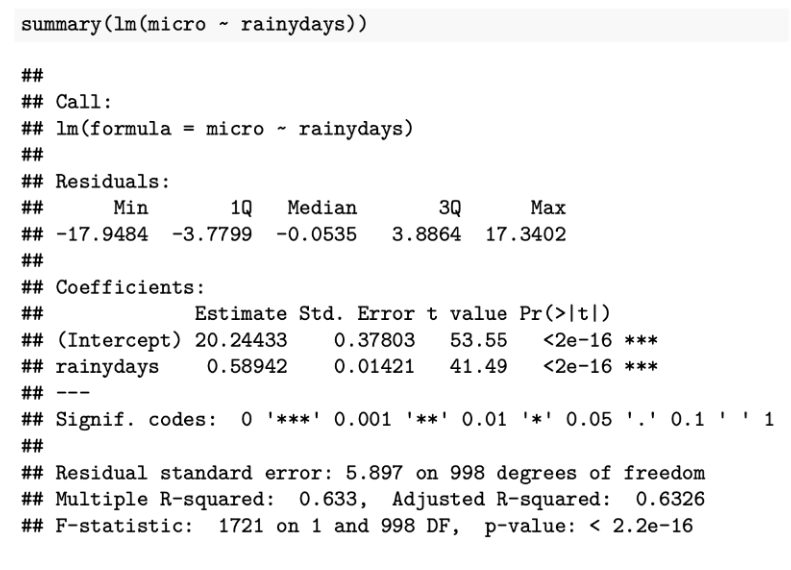
Below is a chunk of code showing a simple linear regression relating the number of pieces of microplastics to the number of days per year with rainfall.

Question 17b raw responses

Respondents submitted a wide variety of answers – responses as they were recorded are included in the tables, below:

Part 6: Programming 1

The following code (in R) defines a function:

compute_turbine_power <- function(height, flowrate, efficiency, maxheight){
  
  if (height < maxheight) {
    
    power = height * flowrate * efficiency
    
  } else {
    
    power = maxheight * flowrate * efficiency
    
  }
  
  return(power)
  
}

This R code applies this function to data:

flowrate = 2
maxheight = 20
power_turbine_a <- compute_turbine_power(10, flowrate, 0.5, maxheight)

Part 7: Environmental Modeling

Part 8: Geospatial Analysis & Remote Sensing

Part 9: Machine Learning

Part 10: Environmental Justice

Part 11: Data Viz & Communication

Identify 4 areas for improvement in the following data visualization that shows information about Michigan counties with highest college attendance (Question 30).

Wordcloud of most frequently occurring words used to describe suggested improvements to the above data visualization (Question 30)

Pre-MEDS

Post-MEDS

Question 30 raw responses

Responses as they were recorded are included in the tables, below:

Part 12: Programming 2

# define function
def convert_F_to_C(temp_F):
  temp_C = (temp_F-32)*5/9
  return temp_C

# use function
convert_F_to_C(32)

End MEDS Class of 2026 PLO Assessment Report

Return to main page

--- title: "MEDS Class of 2026" subtitle: "Program Learning Outcome (PLO) #1 Assessment - Core Knowledge" author: "Sam Shanny-Csik" date: August 13, 2024 date-modified: last-modified format: html: toc: true toc-location: left code-tools: source: true toggle: false theme: - ../styles.scss mainfont: Nunito execute: eval: true echo: false message: false warning: false editor_options: chunk_output_type: console --- ```{r} #..........................load packages......................... library(googlesheets4) library(tidyverse) library(janitor) library(showtext) library(ggtext) library(DT) library(tidytext) library(wordcloud) library(scales) #........................import functions........................ source(here::here("functions.R")) #..........................import data........................... meds2026_before <- read_sheet("https://docs.google.com/spreadsheets/d/1labN4-g9vjaOL96uAg152fQ15rYUiOrfvNgdDGyaJ4A/edit?gid=0#gid=0") # meds2026_after <- read_sheet("") #...........................clean data........................... meds2026_before_clean <- clean_PLO_data(meds2026_before) |> mutate(timepoint = rep("Pre-MEDS")) # meds2026_after_clean <- clean_PLO_data(meds2026_after) |> mutate(timepoint = rep("Post-MEDS")) #...............combine pre- and post-MEDS results............... # both_timepoints_clean <- rbind(meds2026_before_clean, meds2026_after_clean) |> # mutate(timepoint = fct_relevel(timepoint, c("Pre-MEDS", "Post-MEDS"))) #..................number of survey respondents..................= pre_meds_num_respondents <- nrow(meds2026_before_clean) # post_meds_num_respondents <- nrow(meds2026_after_clean) #......................import Google fonts....................... sysfonts::font_add_google(name = "Sanchez", family = "sanchez") sysfonts::font_add_google(name = "Nunito", family = "nunito") # automatically use showtext to render text for future devices ---- showtext::showtext_auto() #......................create color palette...................... 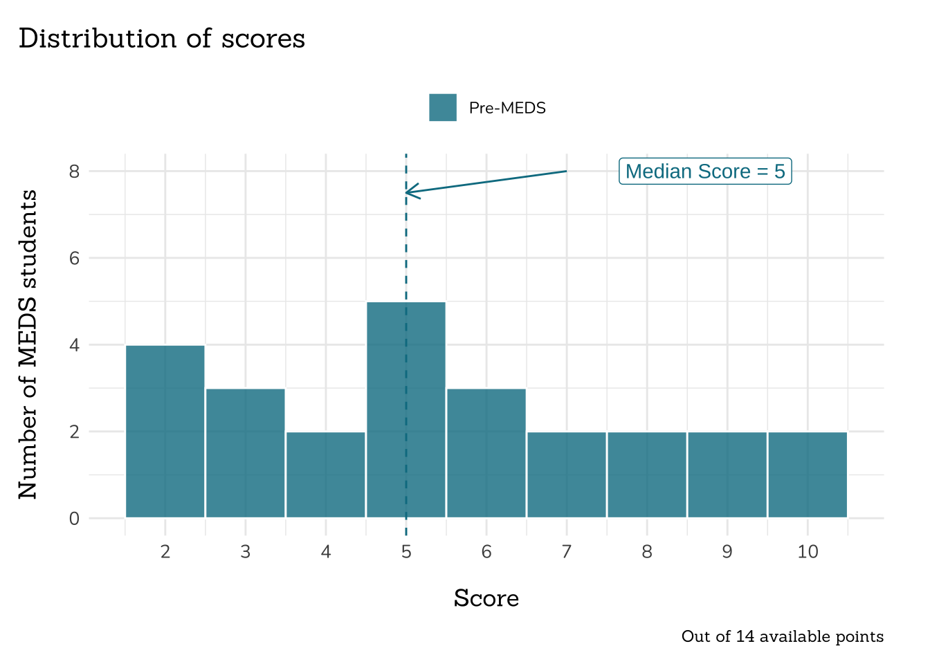meds_pal <- c("Pre-MEDS" = "#047C91", "Post-MEDS" = "#003660") ``` # **Summary**  ```{r overall-scores} #| fig-align: center #........................Pre-MEDS scores......................... scores_before <- meds2026_before_clean |> select(sc0) mean_score_before <- mean(scores_before$sc0) median_score_before <- median(scores_before$sc0) #........................Post-MEDS scores........................ # scores_after <- meds2026_after_clean |> # select(sc0) # mean_score_after <- mean(scores_after$sc0) # median_score_after <- median(scores_after$sc0) #..........................combined plot......................... ggplot(meds2026_before_clean, aes(x = sc0)) + #both_timepoints_clean geom_histogram(aes(fill = timepoint), color = "white", binwidth = 1, position = "identity", alpha = 0.8) + # add "Pre-MEDS" median score ---- geom_vline(xintercept = median_score_before, linetype = "dashed", color = "#047C91") + annotate(geom = "segment", x = 7, y = 8, xend = median_score_before, yend = 7.5, arrow = arrow(length = unit(3, "mm")), color = "#047C91") + annotate(geom = "label", x = 9.8, y = 8, label = paste0("Median Score = ", median_score_before), hjust = "right", color = "#047C91") + # # add "Post-MEDS" median score ---- # geom_vline(xintercept = median_score_after, linetype = "dashed", color = "#003660") + # annotate(geom = "segment", x = 13, y = 8, xend = median_score_after, yend = 7.5, # arrow = arrow(length = unit(3, "mm")), color = "#003660") + # annotate(geom = "label", x = 14, y = 8, # label = paste0("Median Score = ", median_score_after), # hjust = "center", color = "#003660") + # make pretty ---- coord_cartesian(clip = "off") + scale_fill_manual(values = meds_pal) + scale_x_continuous(breaks = seq(1, 14, 1)) + labs(x = "Score", y = "Number of MEDS students", title = "Distribution of scores", caption = "Out of 14 available points") + meds_theme() ``` # **Individual Questions** ## **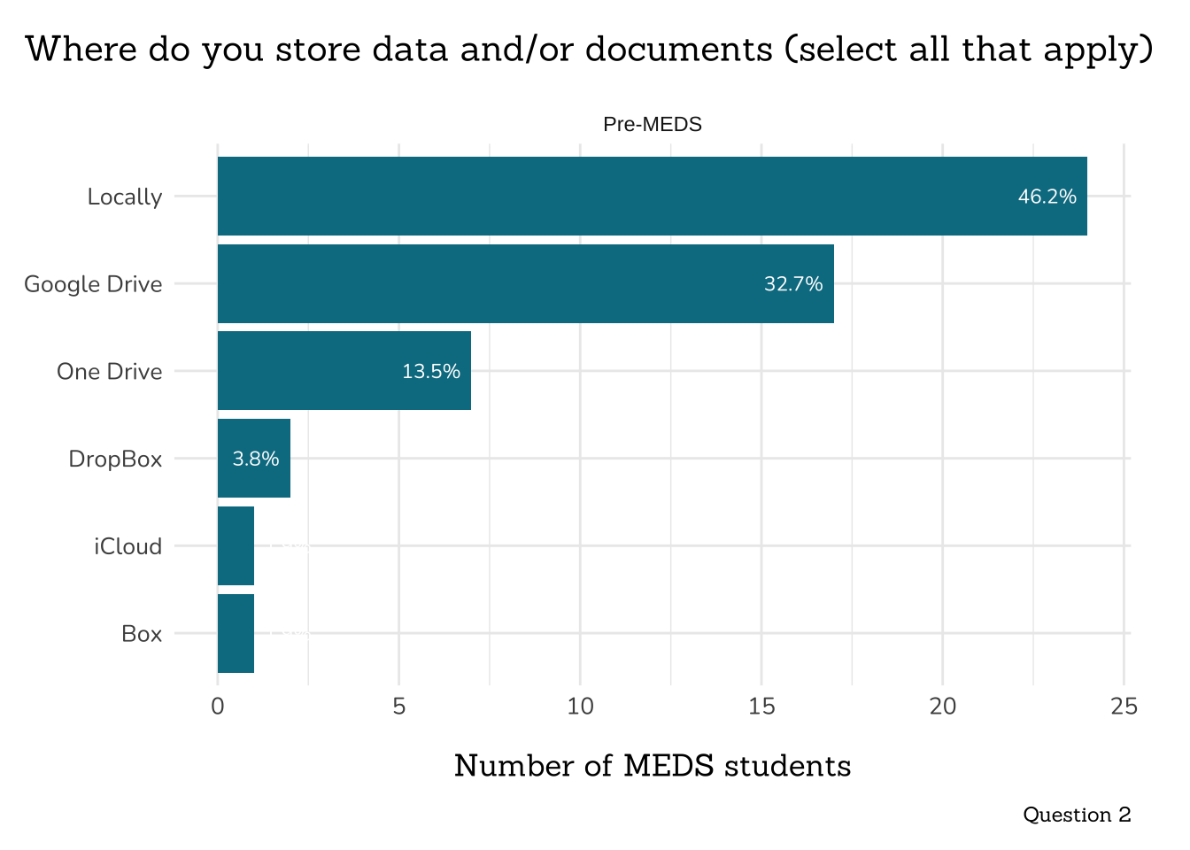Part 1: OS and data/document storage** ```{r Q1-what-OS} ##~~~~~~~~~~~~~~~~~~~~~~~~~~~~~~ ## ~ Question 1: What OS? ---- ##~~~~~~~~~~~~~~~~~~~~~~~~~~~~~~ q1_os_data <- clean_q1_os(meds2026_before_clean) # both_timepoints_clean plot_q1_os(q1_os_data) ``` ```{r Q2-data-storage} #| fig-cap: "NOTE: Percentages will not sum to 100%" ##~~~~~~~~~~~~~~~~~~~~~~~~~~~~~~~~~~~~~~~~~~~~~~ ## ~ Question 2: Where do you store data? ---- ##~~~~~~~~~~~~~~~~~~~~~~~~~~~~~~~~~~~~~~~~~~~~~~ # combine written-in "Other" option responses ---- server <- c("Server", "Taylor server", "external server", "Taylor", "Server", "workbench", "Workbench 1 & 2", "Cyberduck", "server") external_drive <- c("External SSD", "External drive", "external hard drive", "Back up hard drive", "locally on my phone and on my external hard drive", "external ssd, on occasion") icloud <- c("icloud") github <- c("github") locally <- c("Locally on my computer") # wrangle & plot ---- q2_store_data <- clean_q2_store_data(meds2026_before_clean) #both_timepoints_clean plot_q2_store_data(q2_store_data) ``` ## **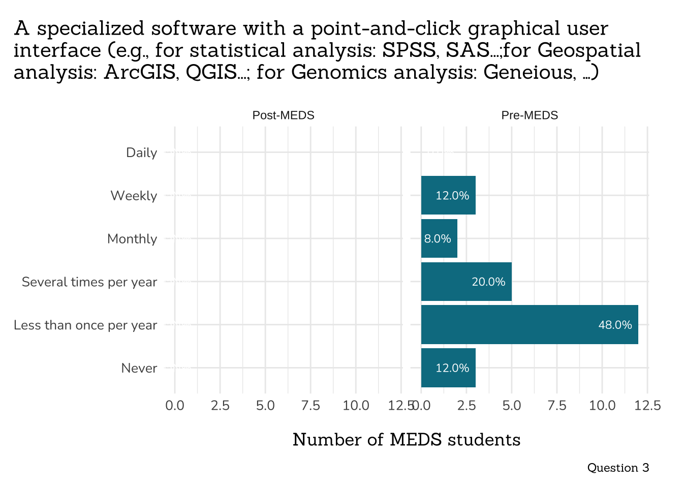Part 2: How often do you currently use the following?** ```{r Q3-GUI} ##~~~~~~~~~~~~~~~~~~~~~~~~~ ## ~ Question 3: GUI ---- ##~~~~~~~~~~~~~~~~~~~~~~~~~ # wrangle ---- q3_gui_data <- clean_freq_rank_data(all_PLO_data = meds2026_before_clean, #both_timepoints_clean, col_name = "point_and_click_gui", categories = c("Never", "Less than once per year", "Several times per year", "Monthly", "Weekly", "Daily")) # plot ---- plot_freq_use_data(data = q3_gui_data, title = "A specialized software with a point-and-click graphical user\ninterface (e.g., for statistical analysis: SPSS, SAS...;for Geospatial\nanalysis: ArcGIS, QGIS...; for Genomics analysis: Geneious, …)", caption = "Question 3") ``` ```{r Q4-prog-lang} ##~~~~~~~~~~~~~~~~~~~~~~~~~~~~~~~~~~~~~~~~~~~ ## ~ Question 4: Programming Languages ---- ##~~~~~~~~~~~~~~~~~~~~~~~~~~~~~~~~~~~~~~~~~~~ # wrangle ---- q4_prog_lang_data <- clean_freq_rank_data(all_PLO_data = meds2026_before_clean,#both_timepoints_clean, col_name = "program_lang", categories = c("Never", "Less than once per year", "Several times per year", "Monthly", "Weekly", "Daily")) # plot ---- plot_freq_use_data(data = q4_prog_lang_data, 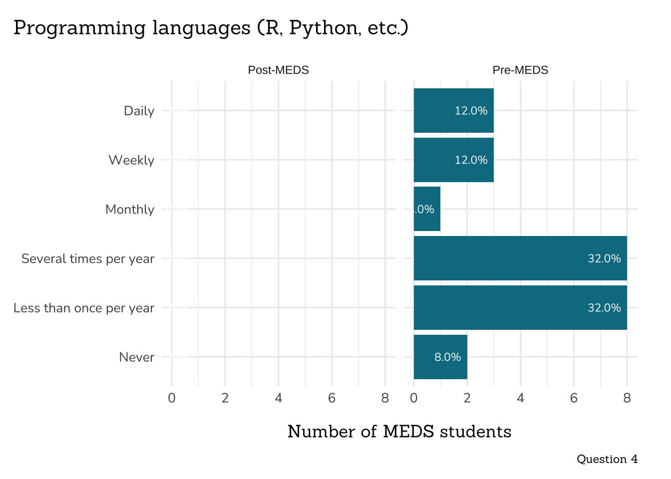title = "Programming languages (R, Python, etc.)", caption = "Question 4") ``` ```{r Q5-databases} ##~~~~~~~~~~~~~~~~~~~~~~~~~~~~~~~ ## ~ Question 5: Databases ---- ##~~~~~~~~~~~~~~~~~~~~~~~~~~~~~~~ # wrangle ---- q5_databases_data <- clean_freq_rank_data(all_PLO_data = meds2026_before_clean, #both_timepoints_clean, col_name = "databases", categories = c("Never", "Less than once per year", "Several times per year", "Monthly", "Weekly", "Daily")) # plot ---- 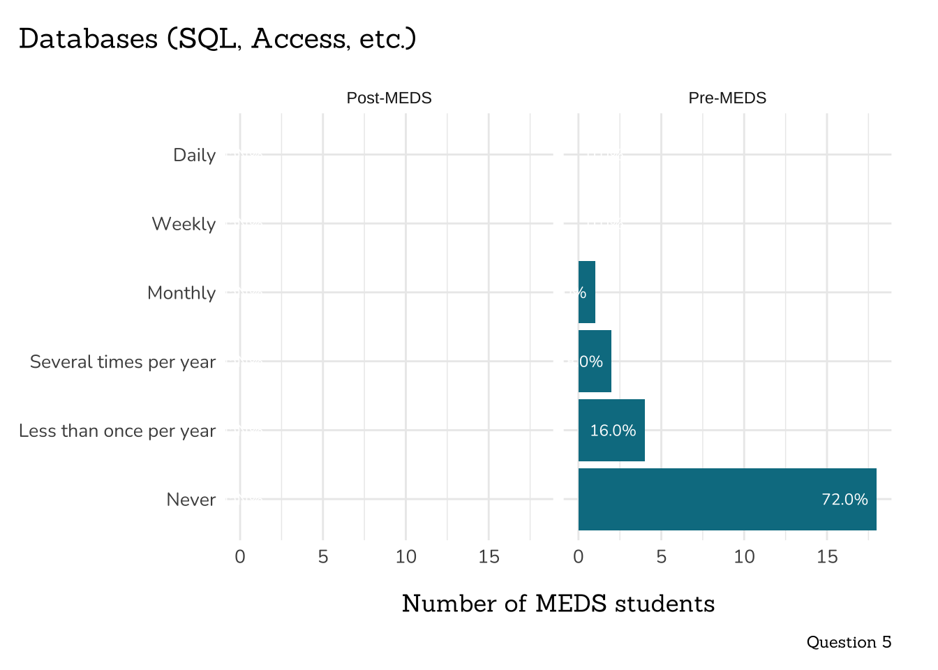plot_freq_use_data(data = q5_databases_data, title = "Databases (SQL, Access, etc.)", caption = "Question 5") ``` ```{r Q6-version-control} ##~~~~~~~~~~~~~~~~~~~~~~~~~~~~~~~~~~~~~ ## ~ Question 6: Version Control ---- ##~~~~~~~~~~~~~~~~~~~~~~~~~~~~~~~~~~~~~ # wrangle ---- q6_version_control_data <- clean_freq_rank_data(all_PLO_data = meds2026_before_clean, #both_timepoints_clean, col_name = "version_control", categories = c("Never", "Less than once per year", "Several times per year", "Monthly", "Weekly", "Daily")) # plot ---- 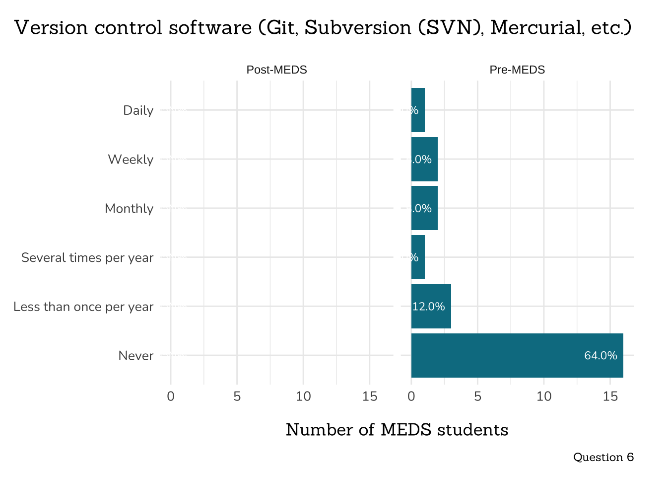plot_freq_use_data(data = q6_version_control_data, title = "Version control software (Git, Subversion (SVN), Mercurial, etc.)", caption = "Question 6") ``` ```{r Q7-command-shell} ##~~~~~~~~~~~~~~~~~~~~~~~~~~~~~~~~~~~ ## ~ Question 7: Command Shell ---- ##~~~~~~~~~~~~~~~~~~~~~~~~~~~~~~~~~~~ # wrangle ---- q7_command_shell_data <- clean_freq_rank_data(all_PLO_data = meds2026_before_clean, #both_timepoints_clean, col_name = "command_shell", categories = c("Never", "Less than once per year", "Several times per year", "Monthly", "Weekly", "Daily")) # plot ---- 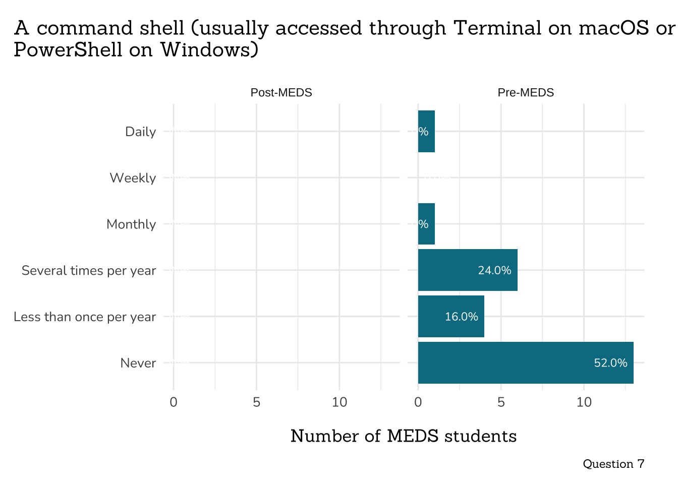plot_freq_use_data(data = q7_command_shell_data, title = "A command shell (usually accessed through Terminal on macOS or\nPowerShell on Windows)", caption = "Question 7") ``` ## **Part 3: Workflow satisfaction** ```{r Q8-workflow-satisfaction} #| results: hide ##~~~~~~~~~~~~~~~~~~~~~~~~~~~~~~~~~~~~~~~~~~~ ## ~ Question 8: Workflow Satisfaction ---- ##~~~~~~~~~~~~~~~~~~~~~~~~~~~~~~~~~~~~~~~~~~~ # wrangle ---- q8_workflow_satisfaction_data <- clean_q8_workflow_sat(meds2026_before_clean) # both_timepoints_clean # plot ---- plot_q8_workflow_sat(q8_workflow_satisfaction_data) ``` ## **Part 4: Rank the following from 1 (strongly disagree) to 5 (strongly agree)** ```{r Q9-raw-data} ##~~~~~~~~~~~~~~~~~~~~~~~~~~~~~~ ## ~ Question 9: Raw Data ---- ##~~~~~~~~~~~~~~~~~~~~~~~~~~~~~~ # wrangle ---- q9_raw_data_data <- clean_freq_rank_data(all_PLO_data = meds2026_before_clean, #both_timepoints_clean, col_name = "raw_data", categories = c("1 (strongly disagree)", "2", "3 (neutral)", "4", "5 (strongly agree)")) # plot ---- 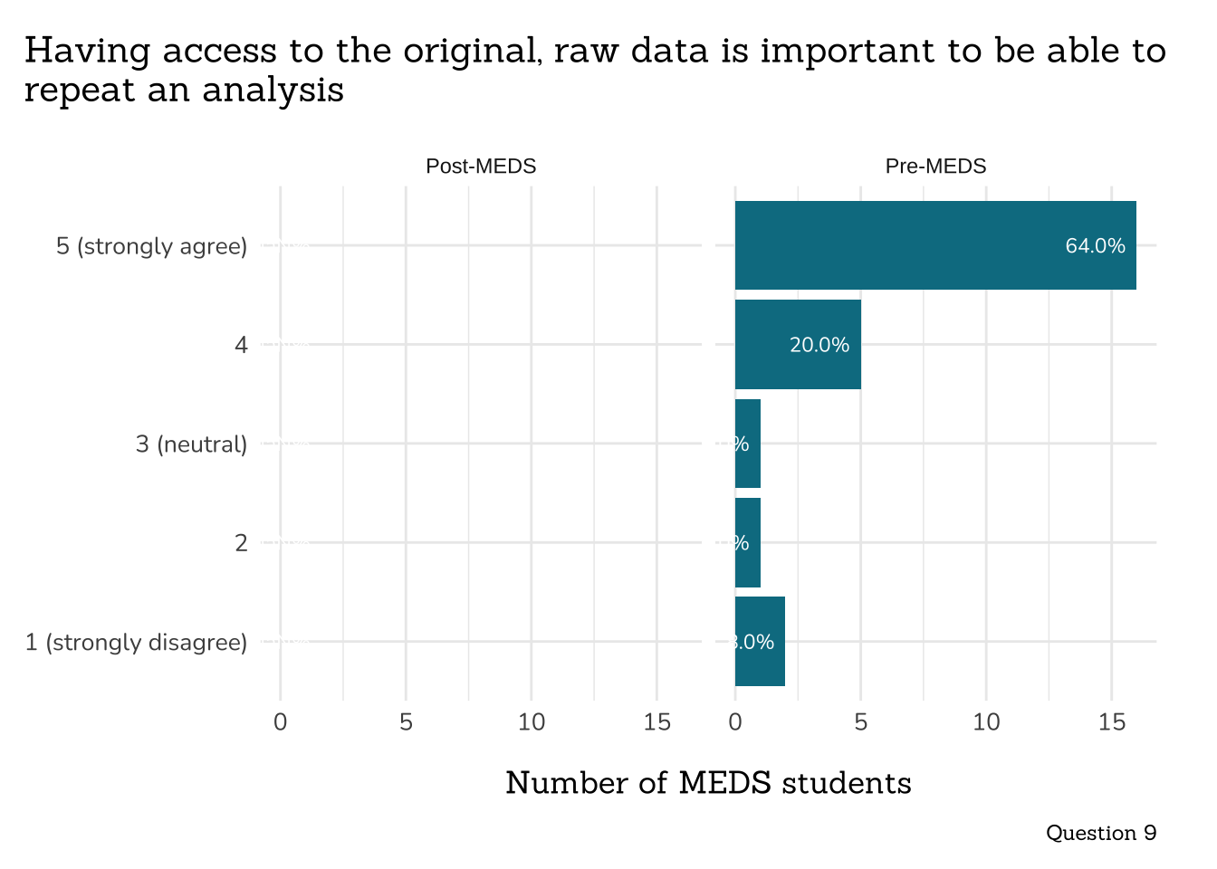plot_rank_data(data = q9_raw_data_data, title = "Having access to the original, raw data is important to be able to\nrepeat an analysis", caption = "Question 9") ``` ```{r Q10-write-script} ##~~~~~~~~~~~~~~~~~~~~~~~~~~~~~~~~~~~~ ## ~ Question 10: Small Program ---- ##~~~~~~~~~~~~~~~~~~~~~~~~~~~~~~~~~~~~ # wrangle ---- q10_small_program_data <- clean_freq_rank_data(all_PLO_data = meds2026_before_clean, #both_timepoints_clean, col_name = "small_program", categories = c("1 (strongly disagree)", "2", "3 (neutral)", "4", "5 (strongly agree)")) # plot ---- plot_rank_data(data = q10_small_program_data, 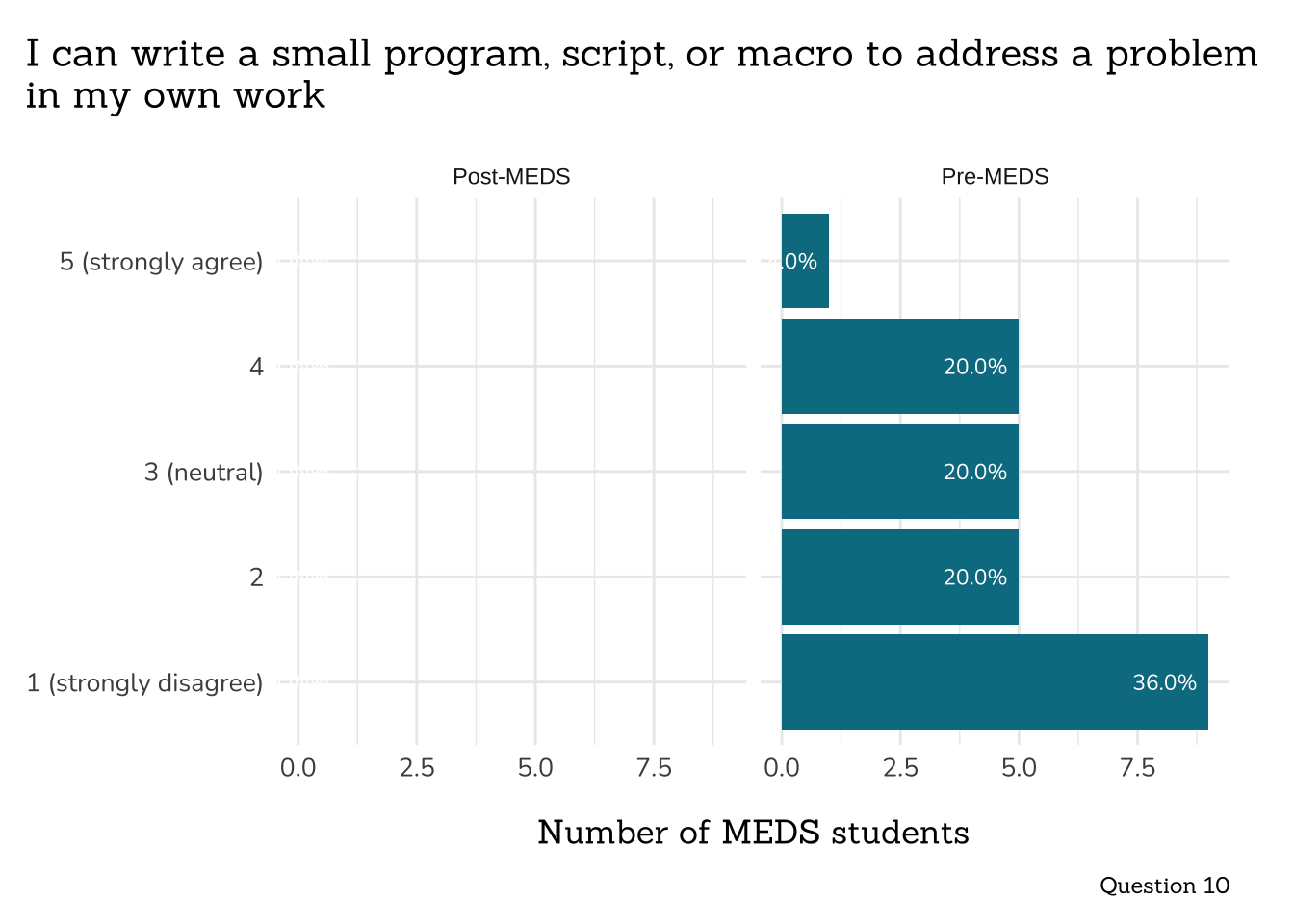title = "I can write a small program, script, or macro to address a problem\nin my own work", caption = "Question 10") ``` ```{r Q11-find-help} ##~~~~~~~~~~~~~~~~~~~~~~~~~~~~~~~~~~~~~~~ ## ~ Question 11: Find Help Online ---- ##~~~~~~~~~~~~~~~~~~~~~~~~~~~~~~~~~~~~~~~ # wrangle ---- q11_find_help_online_data <- clean_freq_rank_data(all_PLO_data = meds2026_before_clean, #both_timepoints_clean, col_name = "find_help_online", categories = c("1 (strongly disagree)", "2", "3 (neutral)", "4", "5 (strongly agree)")) # plot ---- plot_rank_data(data = q11_find_help_online_data , 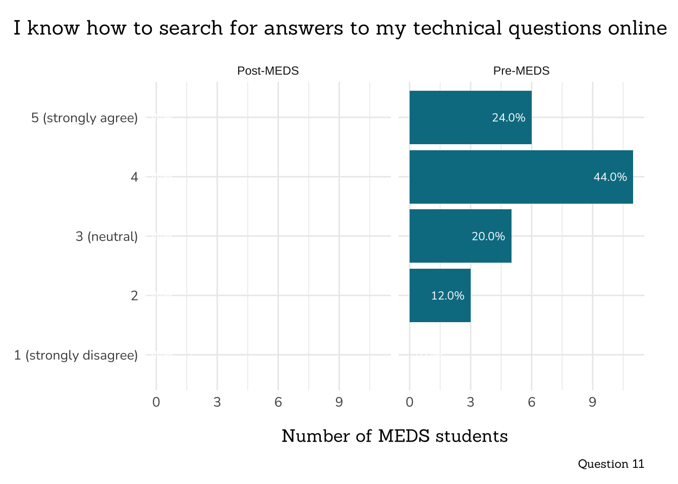title = "I know how to search for answers to my technical questions online", caption = "Question 11") ``` ```{r Q12-overcome-problems} ##~~~~~~~~~~~~~~~~~~~~~~~~~~~~~~~~~~~~~~~~~~ ## ~ Question 12: Overcoming Problems ---- ##~~~~~~~~~~~~~~~~~~~~~~~~~~~~~~~~~~~~~~~~~~ # wrangle ---- q12_overcoming_problems_data <- clean_freq_rank_data(all_PLO_data = meds2026_before_clean, #both_timepoints_clean, col_name = "overcoming_problems", categories = c("1 (strongly disagree)", "2", "3 (neutral)", "4", "5 (strongly agree)")) # plot ---- plot_rank_data(data = q12_overcoming_problems_data, title = "While working on a programming project, if I get stuck, I can find\nways of overcoming the problem", caption = "Question 12") ``` ```{r Q13-confidence} ##~~~~~~~~~~~~~~~~~~~~~~~~~~~~~~~~~ ## ~ Question 13: Confidence ---- ##~~~~~~~~~~~~~~~~~~~~~~~~~~~~~~~~~ # wrangle ---- q13_confidence_data <- clean_freq_rank_data(all_PLO_data = meds2026_before_clean, #both_timepoints_clean, col_name = "confident_programmer", categories = c("1 (strongly disagree)", "2", "3 (neutral)", "4", "5 (strongly agree)")) # plot ---- plot_rank_data(data = q13_confidence_data, 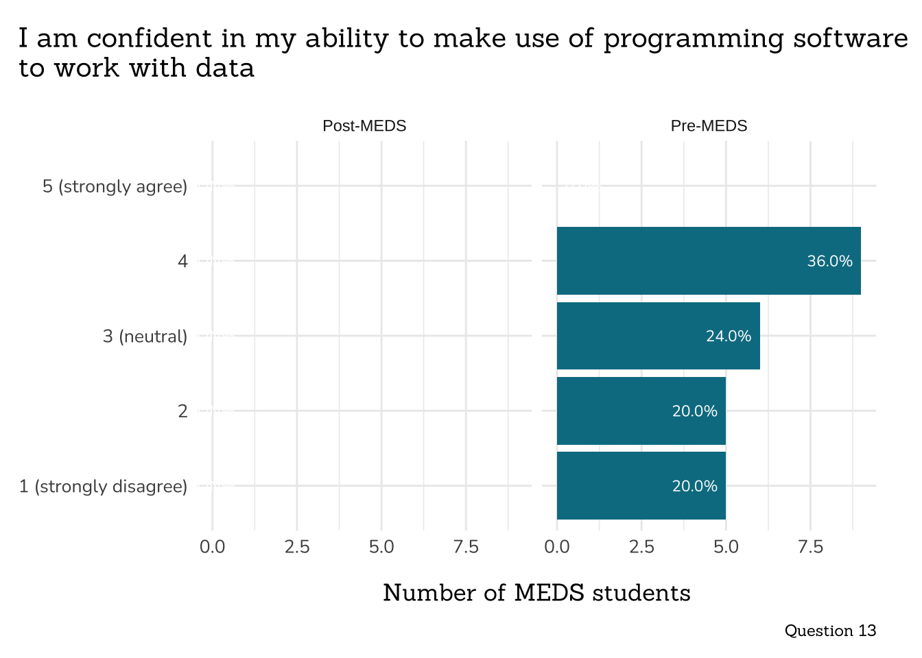title = "I am confident in my ability to make use of programming software\nto work with data", caption = "Question 13") ``` ```{r Q14-easier-analyses} ##~~~~~~~~~~~~~~~~~~~~~~~~~~~~~~~~~~~~~~ ## ~ Question 14: Easier Analyses ---- ##~~~~~~~~~~~~~~~~~~~~~~~~~~~~~~~~~~~~~~ # wrangle ---- q14_easier_analysis_data <- clean_freq_rank_data(all_PLO_data = meds2026_before_clean, #both_timepoints_clean, col_name = "easier_analyses", categories = c("1 (strongly disagree)", "2", "3 (neutral)", "4", "5 (strongly agree)")) # plot ---- plot_rank_data(data = q14_easier_analysis_data, title = "Using a programming language (like R or Python) can make my\nanalyses easier to reproduce", caption = "Question 14") ``` ```{r Q15-increase-efficiency} ##~~~~~~~~~~~~~~~~~~~~~~~~~~~~~~~~~~~~~~~~~~ ## ~ Question 15: Increase Efficiency ---- ##~~~~~~~~~~~~~~~~~~~~~~~~~~~~~~~~~~~~~~~~~~ # wrangle ---- q15_increase_efficiency_data <- clean_freq_rank_data(all_PLO_data = meds2026_before_clean, #both_timepoints_clean, col_name = "increase_efficiency", categories = c("1 (strongly disagree)", "2", "3 (neutral)", "4", "5 (strongly agree)")) # plot ---- plot_rank_data(data = q15_increase_efficiency_data, title = "Using a programming language (like R or Python) can make me\nmore efficient at working with data", caption = "Question 15") ```           ## **Part 5: Stats** ```{r} ##~~~~~~~~~~~~~~~~~~~~~~~~~~~~~~ ## ~ Question 16a: Median ---- ##~~~~~~~~~~~~~~~~~~~~~~~~~~~~~~ # wrangle ---- q16a_median_data <- clean_q16a_median(meds2026_before_clean) #both_timepoints_clean # plot ---- plot_correct_answer_comparison(data = q16a_median_data, 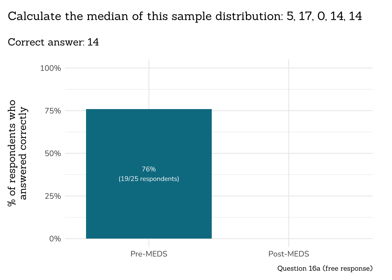title = "Calculate the median of this sample distribution: 5, 17, 0, 14, 14", subtitle = "Correct answer: 14", caption = "Question 16a (free response)") ``` ```{r} ##~~~~~~~~~~~~~~~~~~~~~~~~~~~~ ## ~ Question 16b: Mode ---- ##~~~~~~~~~~~~~~~~~~~~~~~~~~~~ # wrangle ---- q16b_mode_data <- clean_q16b_mode(meds2026_before_clean) #both_timepoints_clean # plot ---- plot_correct_answer_comparison(data = q16b_mode_data, 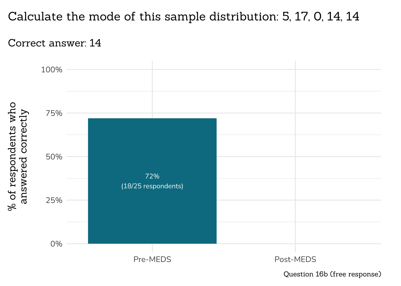title = "Calculate the mode of this sample distribution: 5, 17, 0, 14, 14", subtitle = "Correct answer: 14", caption = "Question 16b (free response)") ``` ```{r} ##~~~~~~~~~~~~~~~~~~~~~~~~~~~~~~~~~~~~~~~~~~~~~~~~~~~~~ ## ~ Question 17a: Linear Regression Familiarity ---- ##~~~~~~~~~~~~~~~~~~~~~~~~~~~~~~~~~~~~~~~~~~~~~~~~~~~~~ # wrangle ---- q17a_familiarity_lr_data <- clean_freq_rank_data(all_PLO_data = meds2026_before_clean, #both_timepoints_clean, col_name = "linear_regression", categories = c("1 - never heard of it", "2", "3 - vague sense of what it means", "4", "5 - very familiar")) # plot ---- plot_rank_data(data = q17a_familiarity_lr_data, 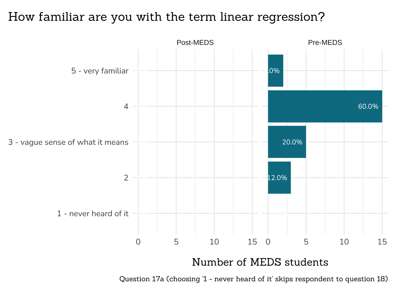title = "How familiar are you with the term linear regression?", caption = "Question 17a (choosing '1 - never heard of it' skips respondent to question 18)") ```  {{< include /summary-text/all_classes/q17b-screenshot.qmd >}} ```{r} ##~~~~~~~~~~~~~~~~~~~~~~~~~~~~~~~~~~~~~ ## ~ Question 17b: Microplastics ---- ##~~~~~~~~~~~~~~~~~~~~~~~~~~~~~~~~~~~~~ # wrangle ---- q17b_microplastics_data <- clean_q17b_microplastics(meds2026_before_clean) # both_timepoints_clean # plot ---- plot_correct_answer_comparison(data = q17b_microplastics_data, 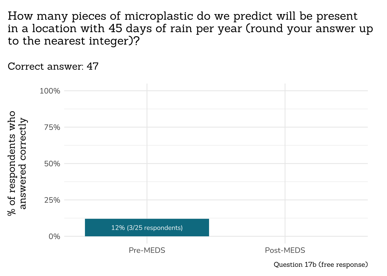title = "How many pieces of microplastic do we predict will be present\nin a location with 45 days of rain per year (round your answer up\nto the nearest integer)?", subtitle = "Correct answer: 47", caption = "Question 17b (free response)") ``` ::: {.callout-note collapse=true} ## Question 17b raw responses Respondents submitted a wide variety of answers -- responses as they were recorded are included in the tables, below: ```{r} ##~~~~~~~~~~~~~~~~~~~~~~~~~~~~~~~~~~~~~~~~~~~~~~~~~~~~~~~~~~~~~~~~~~~~~~~~~~~~~~ ## Pre-MEDS ---- ##~~~~~~~~~~~~~~~~~~~~~~~~~~~~~~~~~~~~~~~~~~~~~~~~~~~~~~~~~~~~~~~~~~~~~~~~~~~~~~ #~..........................wrangle............................. q17_microplastics_dt <- meds2026_before_clean |> #both_timepoints_clean |> # select necessary cols ---- select(timepoint, microplastics_lr) |> # group and count similar responses ---- group_by(timepoint, microplastics_lr) |> count() |> arrange(desc(n)) DT::datatable(q17_microplastics_dt, colnames = c("Timepoint", "Free Response Answer to Q17b", "# of similar responses"), #caption = htmltools::tags$caption( style = 'caption-side: top; text-align: center; color:black; font-size:200% ;','Pre-MEDS:'), options = list(autoWidth = TRUE, pageLength = 5, lengthMenu = c(5, 10, 20, 30), dom = 'ltp') ) ``` ::: ```{r} ##~~~~~~~~~~~~~~~~~~~~~~~~~~~~~~~~~~~~~~~~~~~~~~~~~~~~~~~~~~~~ ## ~ Question 18a: Probability Distribution Familiarity ---- ##~~~~~~~~~~~~~~~~~~~~~~~~~~~~~~~~~~~~~~~~~~~~~~~~~~~~~~~~~~~~ # wrangle ---- q18a_familiar_prob_dist_data <- clean_freq_rank_data(all_PLO_data = meds2026_before_clean, #both_timepoints_clean, col_name = "prob_dist", categories = c("1 (never heard of it)", "2", "3 (vague sense of what it means)", "4", "5 (very familiar)")) # plot ---- 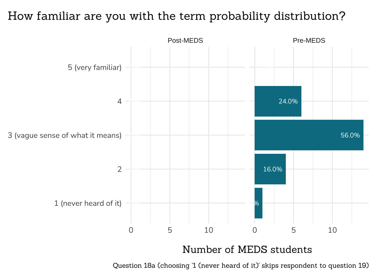plot_rank_data(data = q18a_familiar_prob_dist_data, title = "How familiar are you with the term probability distribution?", caption = "Question 18a (choosing '1 (never heard of it)' skips respondent to question 19)") ```  ```{r} ##~~~~~~~~~~~~~~~~~~~~~~~~~~~~~~~~~~~~~~~~~~~~~~~~~~~~~~~~~~~~~~~~~~~~~~~~~~~~~~ ## Question 18b: Probability Distribution Terms ---- ##~~~~~~~~~~~~~~~~~~~~~~~~~~~~~~~~~~~~~~~~~~~~~~~~~~~~~~~~~~~~~~~~~~~~~~~~~~~~~~ # wrangle (INDIV RESPONSES) ---- q18b_prob_dist_terms_data <- clean_q18b_prob_dist_terms(meds2026_before_clean) #both_timepoints_clean # 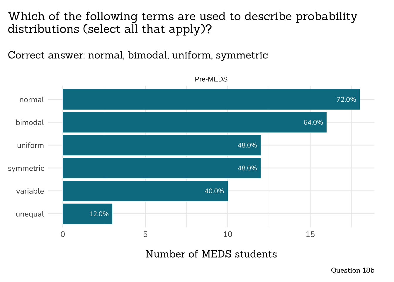plot (INDIV RESPONSES) ---- plot_q18b_prob_dist_terms(q18b_prob_dist_terms_data) ```           ## **Part 6: Programming 1** ```{r} ##~~~~~~~~~~~~~~~~~~~~~~~~~~~~~~~~~~~~~~~~~~~~~~~~~~ ## ~ Question 19a: Familiarity with Functions ---- ##~~~~~~~~~~~~~~~~~~~~~~~~~~~~~~~~~~~~~~~~~~~~~~~~~~ # wrangle ---- q19a_familiar_functions_data <- clean_freq_rank_data(all_PLO_data = meds2026_before_clean, #both_timepoints_clean, col_name = "term_function", categories = c("1 (never heard of it)", "2", "3 (vague sense of what it means)", "4", "5 (very familiar)")) # 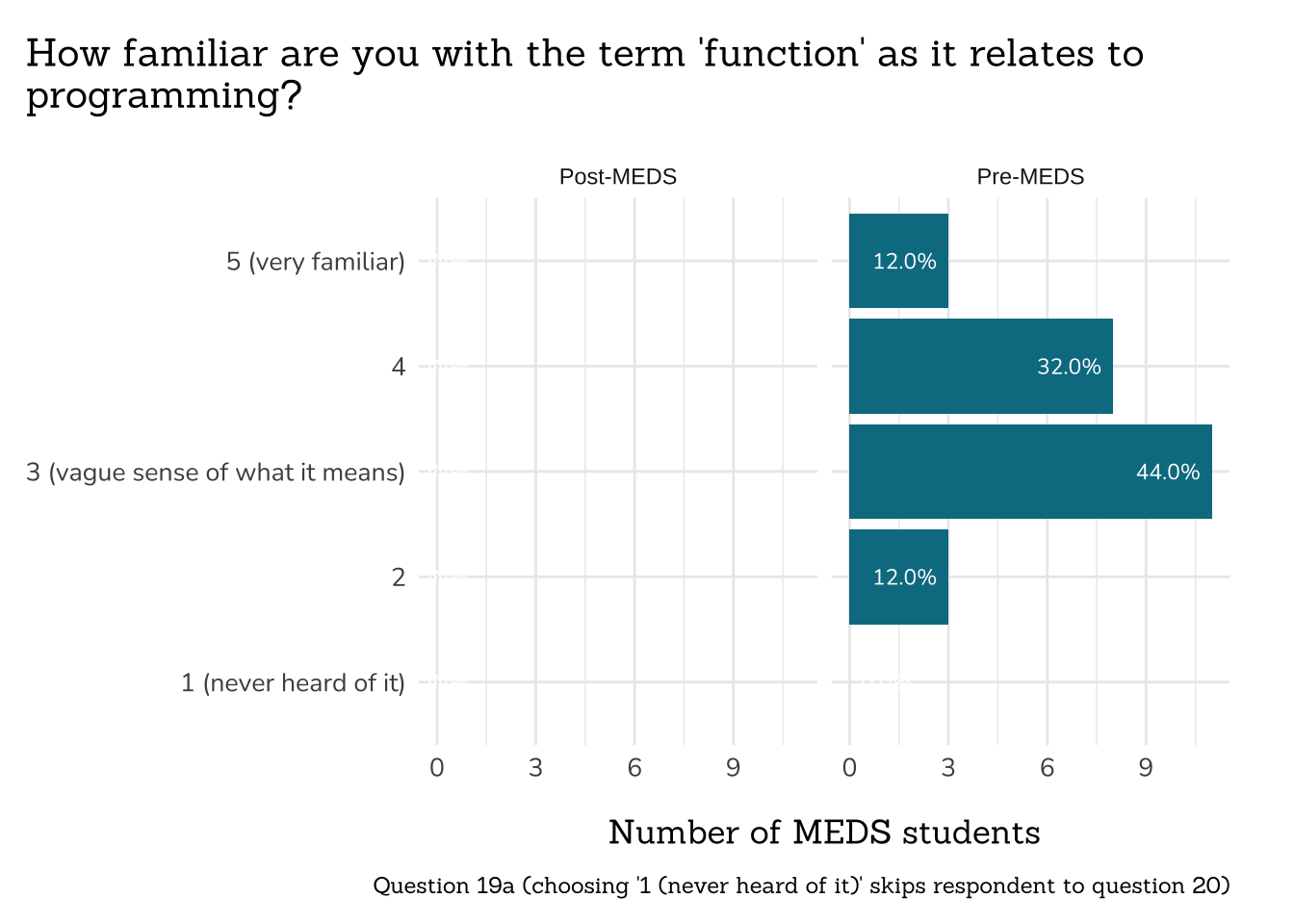plot ---- plot_rank_data(data = q19a_familiar_functions_data, title = "How familiar are you with the term 'function' as it relates to\nprogramming?", caption = "Question 19a (choosing '1 (never heard of it)' skips respondent to question 20)") ```  ```{r} ##~~~~~~~~~~~~~~~~~~~~~~~~~~~~~~~~~~~~~~~~~ ## ~ Question 19b: Writing Functions ---- ##~~~~~~~~~~~~~~~~~~~~~~~~~~~~~~~~~~~~~~~~~ # wrangle ---- q19b_writing_functions_data <- clean_freq_rank_data(all_PLO_data = meds2026_before_clean, # both_timepoints_clean, col_name = "writing_functions", categories = c("1 (not at all comfortable)", "2", "3", "4", "5 (very comfortable)")) # 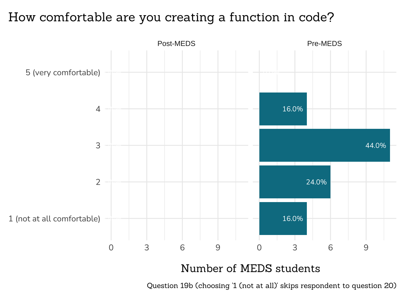plot ---- plot_rank_data(data = q19b_writing_functions_data, title = "How comfortable are you creating a function in code?", caption = "Question 19b (choosing '1 (not at all)' skips respondent to question 20)") ```  {{< 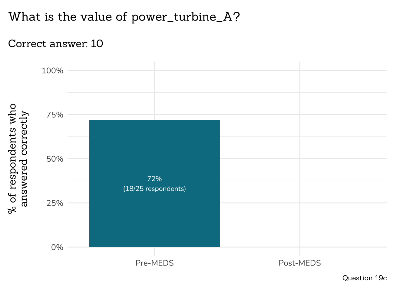include /summary-text/all_classes/q19c-turbine-function.qmd >}} ```{r} ##~~~~~~~~~~~~~~~~~~~~~~~~~~~~~~~~~~~~~~~ ## ~ Question 19c: Function Output ---- ##~~~~~~~~~~~~~~~~~~~~~~~~~~~~~~~~~~~~~~~ # wrangle ---- q19c_fxn_output_data <- clean_q19c_fxn_output(meds2026_before_clean) #both_timepoints_clean # plot ---- plot_correct_answer_comparison(data = q19c_fxn_output_data, title = "What is the value of power_turbine_A?", subtitle = "Correct answer: 10", caption = "Question 19c") ``` ## **Part 7: Environmental Modeling** ```{r} ##~~~~~~~~~~~~~~~~~~~~~~~~~~~~~~~~~~~~~~~~~~~~~~~ ## ~ Question 20a: Run Environmental Model ---- ##~~~~~~~~~~~~~~~~~~~~~~~~~~~~~~~~~~~~~~~~~~~~~~~ # wrangle ---- 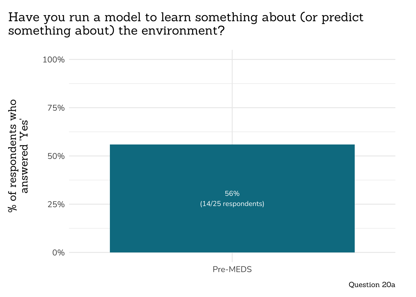q20a_run_env_mod_data <- clean_q20a_run_env_mod(meds2026_before_clean) #both_timepoints_clean # plot ---- plot_q20a_run_env_mod(q20a_run_env_mod_data) ```  ```{r} ##~~~~~~~~~~~~~~~~~~~~~~~~~~~~~~~~~~~~~~~~~~~~ ## ~ Question 20b: Sensitivity Analysis ---- ##~~~~~~~~~~~~~~~~~~~~~~~~~~~~~~~~~~~~~~~~~~~~ # wrangle ---- 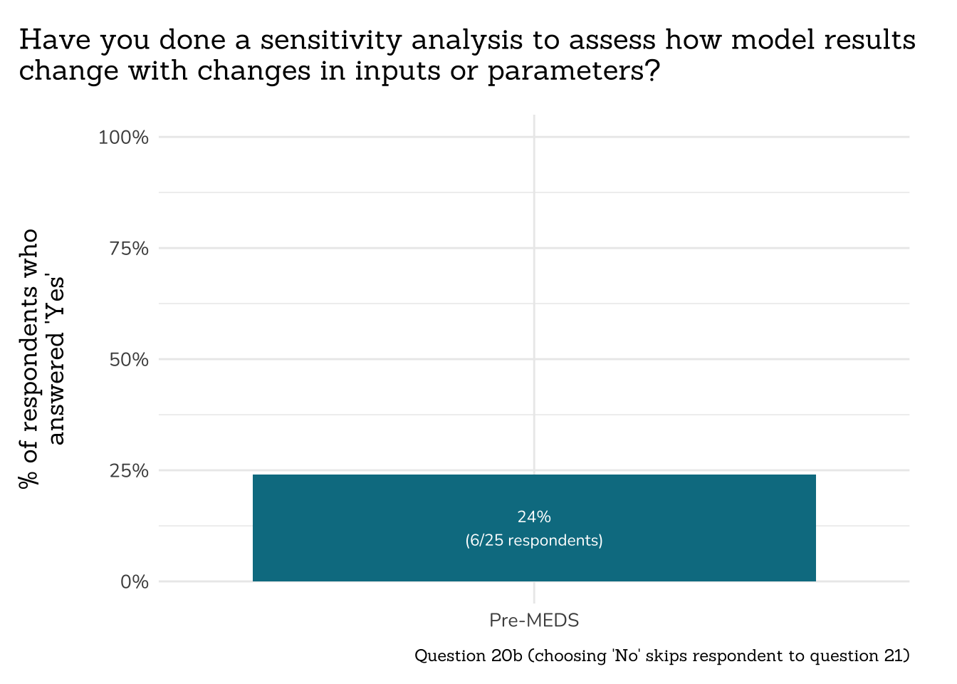q20b_sa_data <- clean_q20b_sa(meds2026_before_clean) #both_timepoints_clean # plot ---- plot_q20b_sa(q20b_sa_data) ```  ```{r} ##~~~~~~~~~~~~~~~~~~~~~~~~~~~~~~~~~~~~~~~~~~~~~~ ## ~ Question 20c: Parameter Interactions ---- ##~~~~~~~~~~~~~~~~~~~~~~~~~~~~~~~~~~~~~~~~~~~~~~ # wrangle ---- 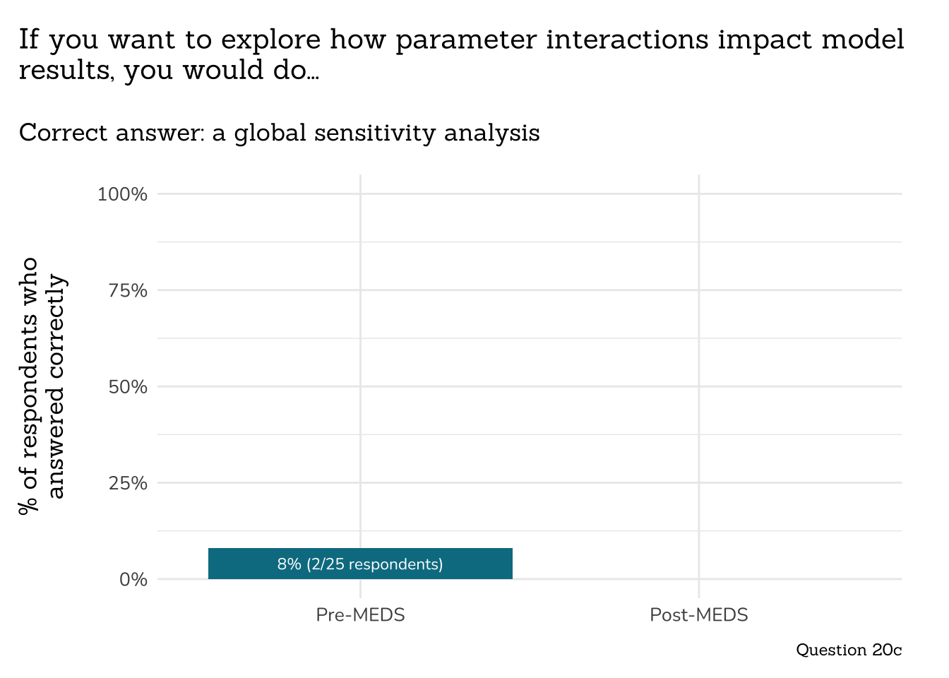q20c_param_int_data <- clean_q20c_param_int(meds2026_before_clean) # both_timepoints_clean # plot ---- plot_correct_answer_comparison(data = q20c_param_int_data, title = "If you want to explore how parameter interactions impact model\nresults, you would do...", subtitle = "Correct answer: a global sensitivity analysis", caption = "Question 20c") ``` ## **Part 8: Geospatial Analysis & Remote Sensing** ```{r} ##~~~~~~~~~~~~~~~~~~~~~~~~~~~~~~~~~~~~~~~~~~~~~~~~~ ## ~ Question 21a: Comfort with Spatial Data ---- ##~~~~~~~~~~~~~~~~~~~~~~~~~~~~~~~~~~~~~~~~~~~~~~~~~ # wrangle ---- q21a_comfort_spatial_data <- clean_freq_rank_data(all_PLO_data = meds2026_before_clean, #both_timepoints_clean, col_name = "spatial_data", categories = c("1 (never worked with it before)", "2", "3", "4", "5 (work with it all the time)")) # plot ---- 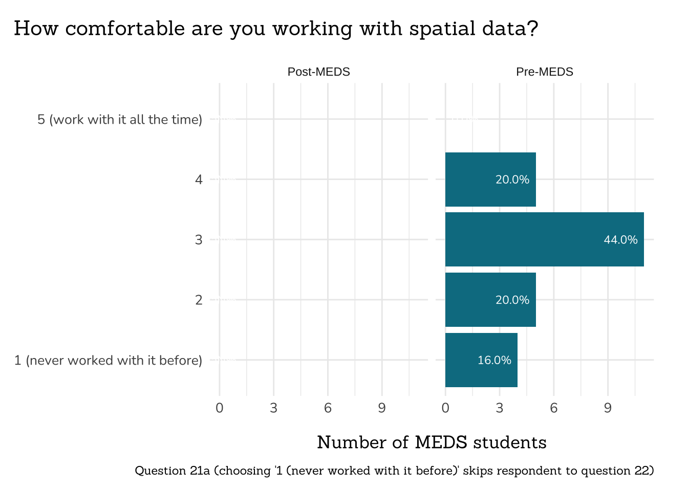plot_rank_data(data = q21a_comfort_spatial_data, title = "How comfortable are you working with spatial data?", caption = "Question 21a (choosing '1 (never worked with it before)' skips respondent to question 22)") ```  ```{r} # wrangle (INDIV RESPONSES) ---- 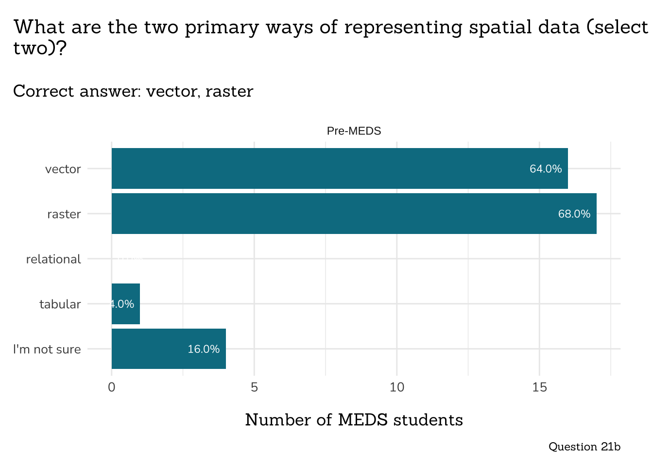q21b_rep_spatial_data <- clean_q21b_rep_spatial(meds2026_before_clean) # both_timepoints_clean # plot (INDIV RESPONSES) ---- plot_q21b_rep_spatial(q21b_rep_spatial_data) ```         ```{r} ##~~~~~~~~~~~~~~~~~~~~~~~~~~~~~~~~~~~~~~~~~ ## ~ Question 21c: Vector vs. 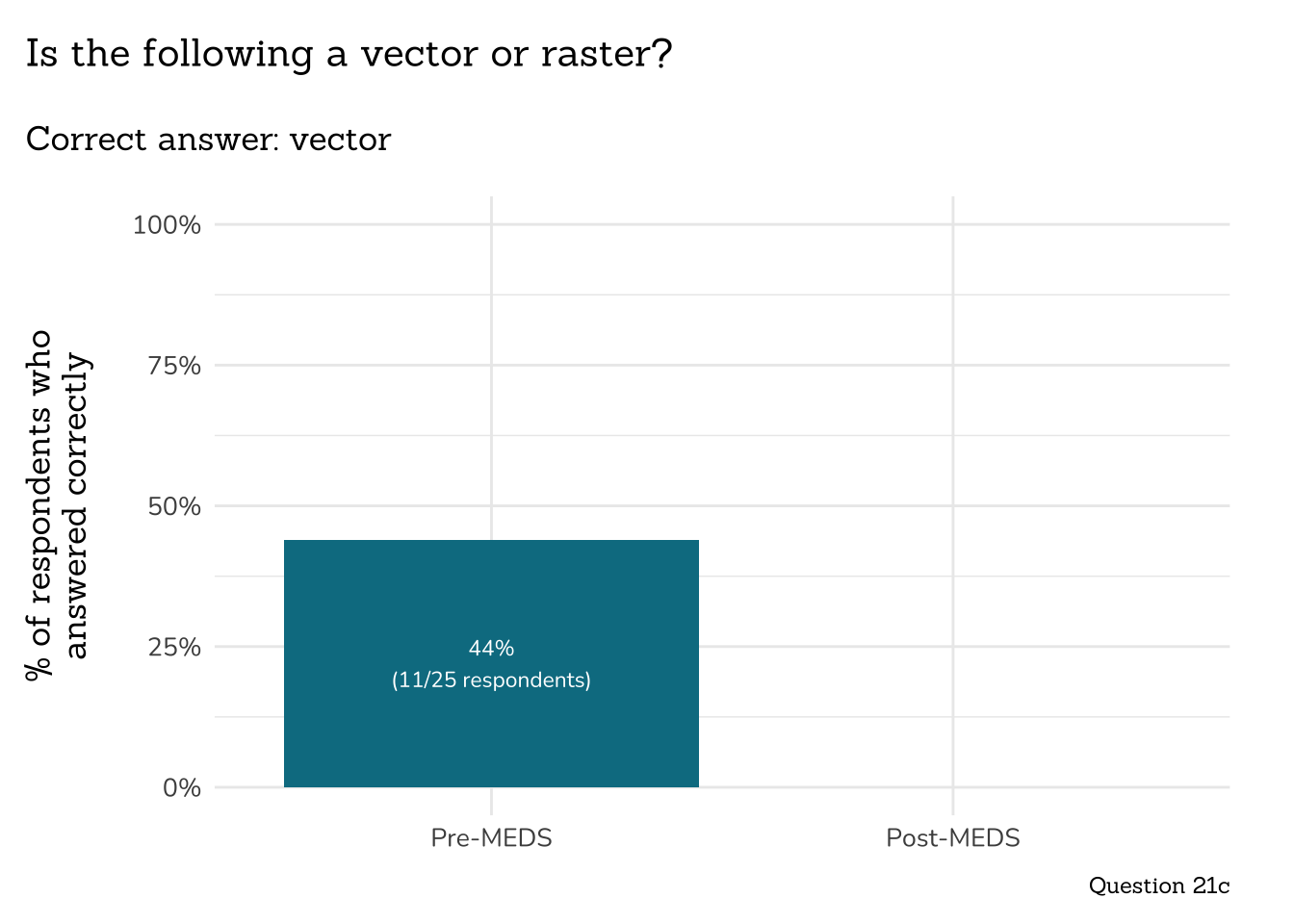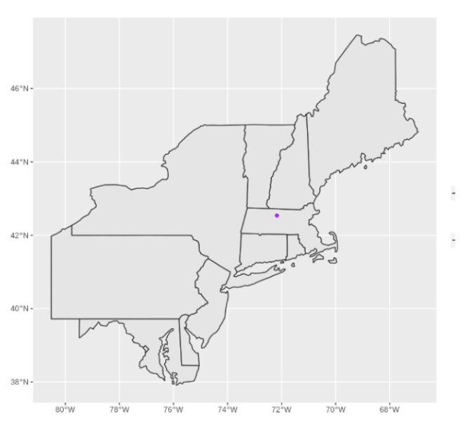Raster ---- ##~~~~~~~~~~~~~~~~~~~~~~~~~~~~~~~~~~~~~~~~~ # wrangle ---- q21c_vec_ras_data <- clean_q21c_vec_ras(meds2026_before_clean) # both_timepoints_clean # plot ---- plot_correct_answer_comparison(data = q21c_vec_ras_data, title = "Is the following a vector or raster?", subtitle = "Correct answer: vector", caption = "Question 21c") ``` ```{r} #| fig-align: center knitr::include_graphics(here::here("yearly-reports", "images", "21c-vector.png")) ``` ```{r} ##~~~~~~~~~~~~~~~~~~~~~~~~~~~~~~~~~~~~~~~~~~~~~~~~~~~ ## ~ Question 22a: Comfort with Remote Sensing ---- ##~~~~~~~~~~~~~~~~~~~~~~~~~~~~~~~~~~~~~~~~~~~~~~~~~~~ # wrangle ---- q22a_comfort_rs_data <- clean_freq_rank_data(all_PLO_data = meds2026_before_clean, # both_timepoints_clean, col_name = "remote_sense_comfort", categories = c("1 (never worked with it before)", "2", "3", "4", "5 (work with it all the time)")) # plot ---- 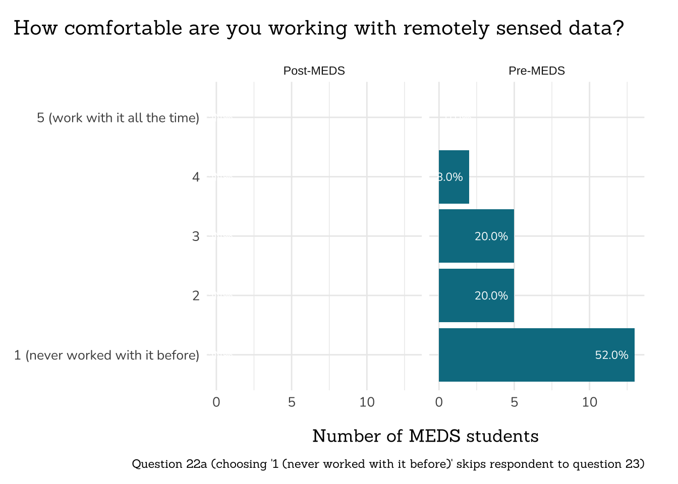plot_rank_data(data = q22a_comfort_rs_data, title = "How comfortable are you working with remotely sensed data?", caption = "Question 22a (choosing '1 (never worked with it before)' skips respondent to question 23)") ```  ```{r} ##~~~~~~~~~~~~~~~~~~~~~~~~~~~~~~~~~~~~~~~~~~~ ## ~ Question 22b: Reflected Radiation ---- ##~~~~~~~~~~~~~~~~~~~~~~~~~~~~~~~~~~~~~~~~~~~ # wrangle ---- q22b_rs_sun_data <- clean_q22b_rs_sun(meds2026_before_clean) #both_timepoints_clean # plot ---- 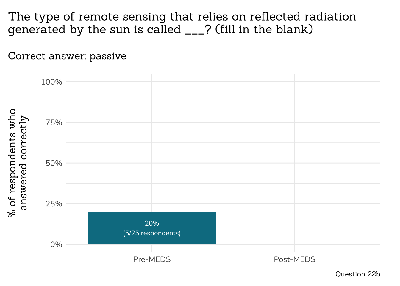plot_correct_answer_comparison(data = q22b_rs_sun_data, title = "The type of remote sensing that relies on reflected radiation\ngenerated by the sun is called ___? (fill in the blank)", subtitle = "Correct answer: passive", caption = "Question 22b") ``` ```{r} ##~~~~~~~~~~~~~~~~~~~~~~~~~~~~~~~~~~~~~~~ ## ~ Question 23a: Map Projections ---- ##~~~~~~~~~~~~~~~~~~~~~~~~~~~~~~~~~~~~~~~ # wrangle ---- q23a_comfort_map_proj_data <- clean_freq_rank_data(all_PLO_data = meds2026_before_clean, #both_timepoints_clean, col_name = "map_proj_comfort", categories = c("1 (never worked with it before)", "2", "3", "4", "5 (work it with all the time)")) # plot ---- 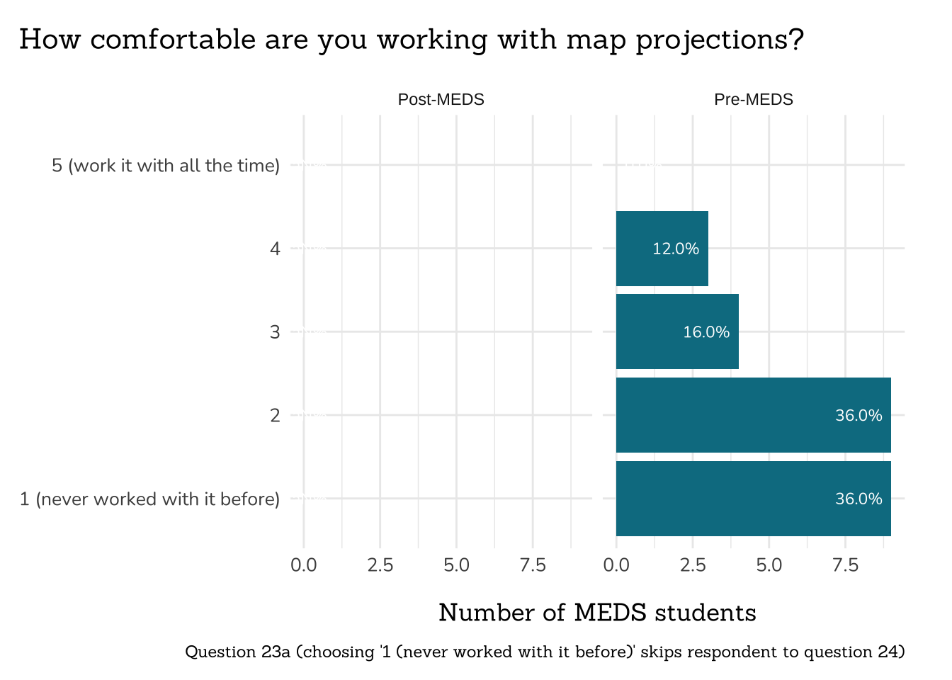plot_rank_data(data = q23a_comfort_map_proj_data, title = "How comfortable are you working with map projections?", caption = "Question 23a (choosing '1 (never worked with it before)' skips respondent to question 24)") ```  ```{r} ##~~~~~~~~~~~~~~~~~~~~~~~~~~~~~~~~~~~~ ## ~ Question 23b: Reprojection ---- ##~~~~~~~~~~~~~~~~~~~~~~~~~~~~~~~~~~~~ # wrangle ---- q23b_reproj_data <- clean_q23b_reproj(meds2026_before_clean) # both_timepoints_clean # plot ---- 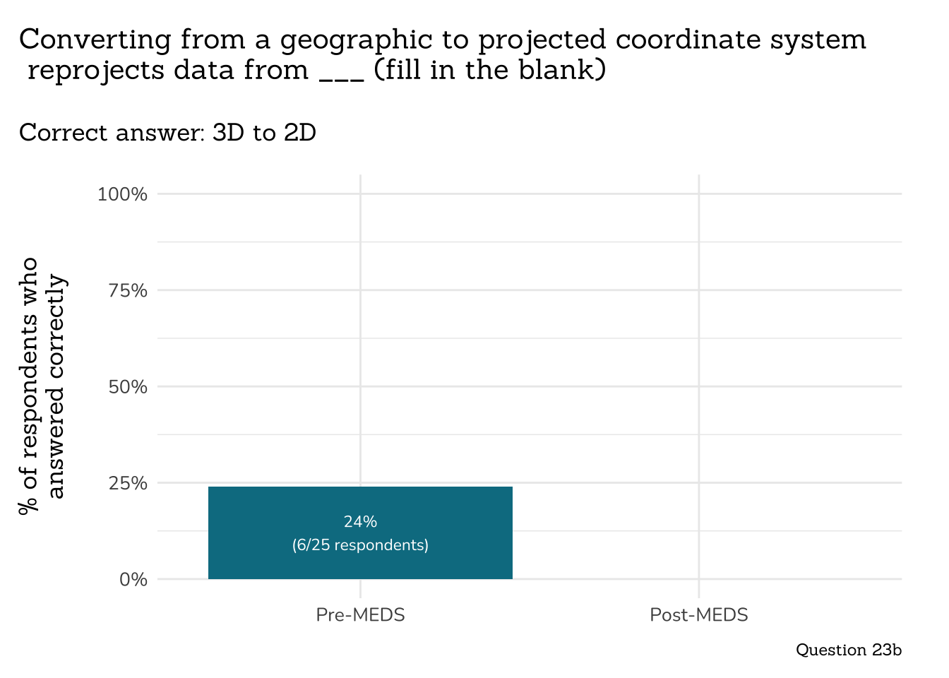plot_correct_answer_comparison(data = q23b_reproj_data, title = "Converting from a geographic to projected coordinate system\n reprojects data from ___ (fill in the blank)", subtitle = "Correct answer: 3D to 2D", caption = "Question 23b") ``` ```{r} ##~~~~~~~~~~~~~~~~~~~~~~~~~~~~~~~~~~~~~~~~~~~~~~~~~~~~~~~~~~~~ ## ~ Question 24a: Familiarity with Reflectance Spectra ---- ##~~~~~~~~~~~~~~~~~~~~~~~~~~~~~~~~~~~~~~~~~~~~~~~~~~~~~~~~~~~~ # wrangle ---- q24a_familiarity_rs_data <- clean_freq_rank_data(all_PLO_data = meds2026_before_clean, # both_timepoints_clean, col_name = "reflec_spec", categories = c("1 (never heard of it)", "2", "3 (vague sense of what it means)", "4", "5 (very familiar)")) # plot ---- 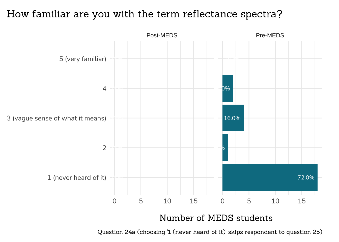plot_rank_data(data = q24a_familiarity_rs_data, title = "How familiar are you with the term reflectance spectra?", caption = "Question 24a (choosing '1 (never heard of it)' skips respondent to question 25)") ```  ```{r} ##~~~~~~~~~~~~~~~~~~~~~~~~~~~~~~~~~~~~~~~~~~~~~ ## ~ Question 24b: Vegetation Wavelength ---- ##~~~~~~~~~~~~~~~~~~~~~~~~~~~~~~~~~~~~~~~~~~~~~ # wrangle ---- q24b_veg_wave_data <- clean_q24b_veg_wave(meds2026_before_clean) # both_timepoints_clean # plot ---- 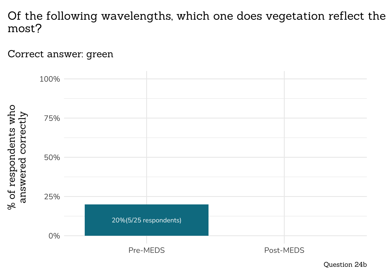plot_correct_answer_comparison(data = q24b_veg_wave_data, title = "Of the following wavelengths, which one does vegetation reflect the\nmost?", subtitle = "Correct answer: green", caption = "Question 24b") ``` ## **Part 9: Machine Learning** ```{r} ##~~~~~~~~~~~~~~~~~~~~~~~~~~~~~~~~~~~~~~~~~~~ ## ~ Question 25a: Familiarity with ML ---- ##~~~~~~~~~~~~~~~~~~~~~~~~~~~~~~~~~~~~~~~~~~~ # wrangle ---- q25a_familiar_ml_data <- clean_freq_rank_data(all_PLO_data = meds2026_before_clean, #both_timepoints_clean, col_name = "sup_vs_unsup_learn", categories = c("1 (never heard of either of those terms)", "2", "3 (vague sense of these terms, but not why they are distinct from one another)", "4", "5 (very familiar with both concepts and how they differ)")) # plot ---- 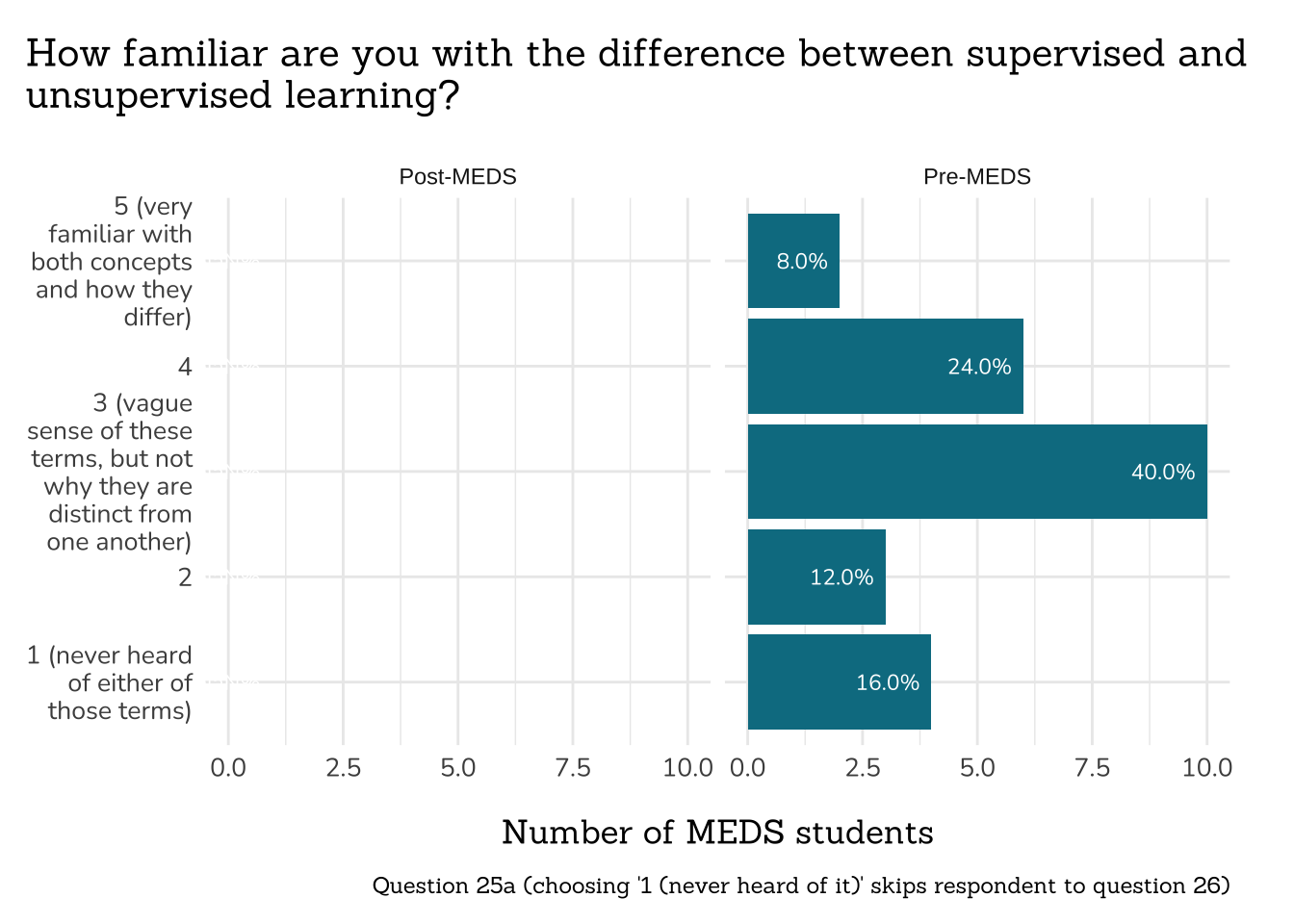plot_rank_data(data = q25a_familiar_ml_data, title = "How familiar are you with the difference between supervised and\nunsupervised learning?", caption = "Question 25a (choosing '1 (never heard of it)' skips respondent to question 26)") + scale_x_discrete(labels = function(x) str_wrap(x, width = 15)) ```  ```{r} ##~~~~~~~~~~~~~~~~~~~~~~~~~~~~~~~~~~~~~~~~~~~~~~~~~~~~~~~ ## ~ Question 25b: Unsupervised Learning Algorithm ---- ##~~~~~~~~~~~~~~~~~~~~~~~~~~~~~~~~~~~~~~~~~~~~~~~~~~~~~~~ # wrangle ---- q25b_unsup_alg_data <- clean_freq_rank_data(all_PLO_data = meds2026_before_clean, #both_timepoints_clean, col_name = "implemented_algo", categories = c("1 (definitely not)", "2", "3 (maybe, but I'm not sure)", "4", "5 (yes)")) |> filter(xvar != "NULL") # plot ---- 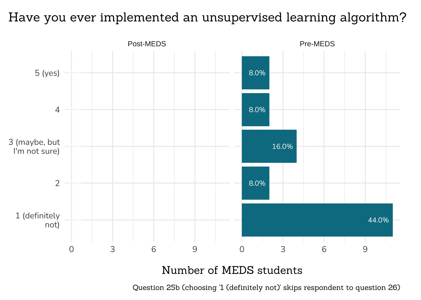plot_rank_data(data = q25b_unsup_alg_data, title = "Have you ever implemented an unsupervised learning algorithm?", caption = "Question 25b (choosing '1 (definitely not)' skips respondent to question 26)") + scale_x_discrete(labels = function(x) str_wrap(x, width = 15)) ```  ```{r} ##~~~~~~~~~~~~~~~~~~~~~~~~~~~~~~ ## ~ Question 25c: Kmeans ---- ##~~~~~~~~~~~~~~~~~~~~~~~~~~~~~~ # wrangle ---- q25c_kmeans_data <- clean_q25c_kmeans(meds2026_before_clean) # both_timepoints_clean # plot ---- 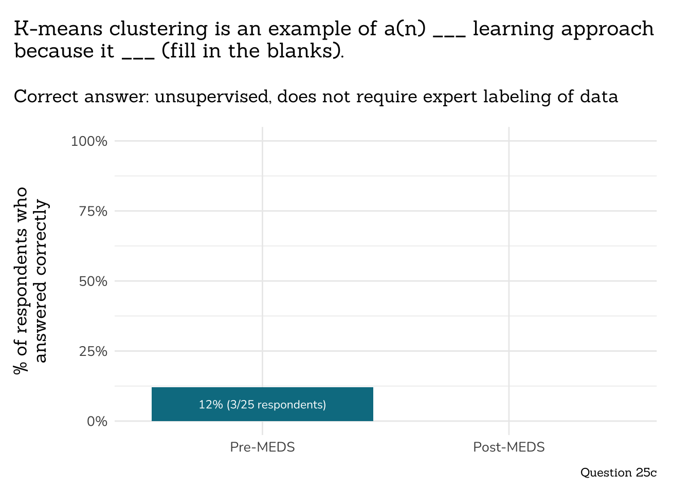plot_correct_answer_comparison(data = q25c_kmeans_data, title = "K-means clustering is an example of a(n) ___ learning approach\nbecause it ___ (fill in the blanks).", subtitle = "Correct answer: unsupervised, does not require expert labeling of data", caption = "Question 25c") ``` ```{r} ##~~~~~~~~~~~~~~~~~~~~~~~~~~~~~~~~~~~~~ ## ~ Question 26a: Dividing Data ---- ##~~~~~~~~~~~~~~~~~~~~~~~~~~~~~~~~~~~~~ # wrangle ---- q26a_div_data <- clean_freq_rank_data(all_PLO_data = meds2026_before_clean, #both_timepoints_clean, col_name = "ml_div_data", categories = c("1 (never heard of it)", "2", "3 (vague sense of what it means)", "4", "5 (very familiar)")) # plot ---- 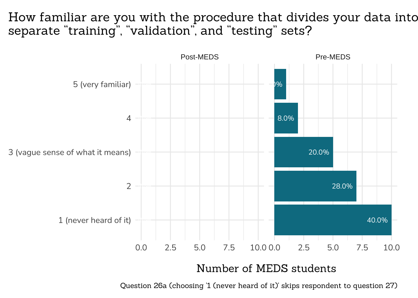plot_rank_data(data = q26a_div_data, title = "How familiar are you with the procedure that divides your data into\nseparate “training”, “validation”, and “testing” sets?", caption = "Question 26a (choosing '1 (never heard of it)' skips respondent to question 27)") ```  ```{r} ##~~~~~~~~~~~~~~~~~~~~~~~~~~~~~~~~~~~~~~~~~~~~~~ ## ~ Question 26b: Train, Validate, Split ---- ##~~~~~~~~~~~~~~~~~~~~~~~~~~~~~~~~~~~~~~~~~~~~~~ # wrangle ---- q26b_tvs_data <- clean_freq_rank_data(all_PLO_data = meds2026_before_clean, # both_timepoints_clean, col_name = "train_valid_split", categories = c("1 (never)", "2", "3", "4", "5 (all the time)")) |> filter(xvar != "NULL") # plot ---- 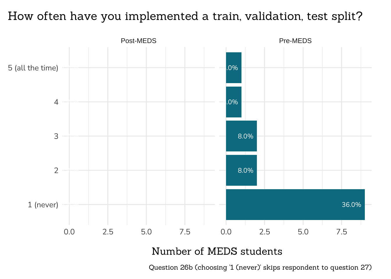plot_rank_data(data = q26b_tvs_data, title = "How often have you implemented a train, validation, test split?", caption = "Question 26b (choosing '1 (never)' skips respondent to question 27)") ```  ```{r} # wrangle (INDIV RESPONSES) ---- 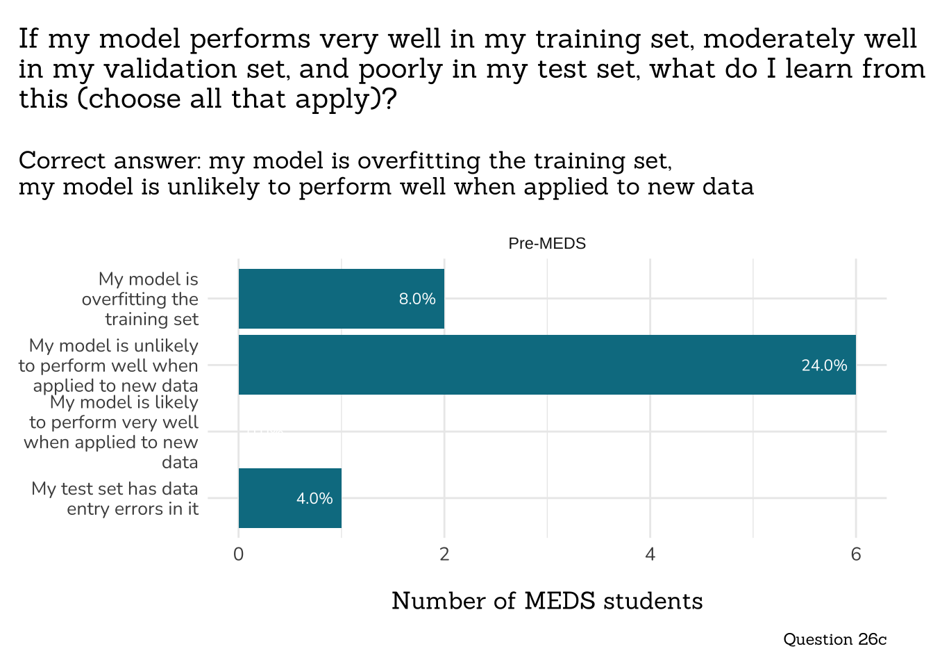q26c_mod_perf_data <- clean_q26c_mod_perf(meds2026_before_clean) # both_timepoints_clean # plot (INDIV RESPONSES) ---- plot_q26c_mod_perf(q26c_mod_perf_data) ```           ## **Part 10: Environmental Justice** ```{r} ##~~~~~~~~~~~~~~~~~~~~~~~~~~~~~~~~~~~ ## ~ Question 27: Data Justice ---- ##~~~~~~~~~~~~~~~~~~~~~~~~~~~~~~~~~~~ # wrangle ---- q27_data_justice_data <- clean_freq_rank_data(all_PLO_data = meds2026_before_clean, # both_timepoints_clean, col_name = "data_justice", categories = c("1 (never heard of it)", "2", "3 (vague sense of what it means)", "4", "5 (very familiar)")) # plot ---- 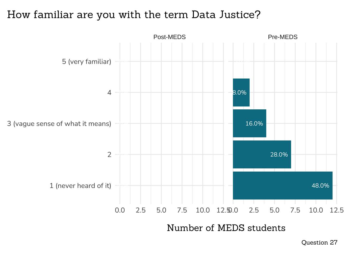plot_rank_data(data = q27_data_justice_data, title = "How familiar are you with the term Data Justice?", caption = "Question 27") ``` ```{r} ##~~~~~~~~~~~~~~~~~~~~~~~~~~~ ## ~ Question 28: Bias ---- ##~~~~~~~~~~~~~~~~~~~~~~~~~~~ # wrangle ---- q28_bias_data <- clean_freq_rank_data(all_PLO_data = meds2026_before_clean, # both_timepoints_clean, col_name = "bias", categories = c("1 (strongly disagree)", "2", "3 (neutral)", "4", "5 (strongly agree)")) # plot ---- 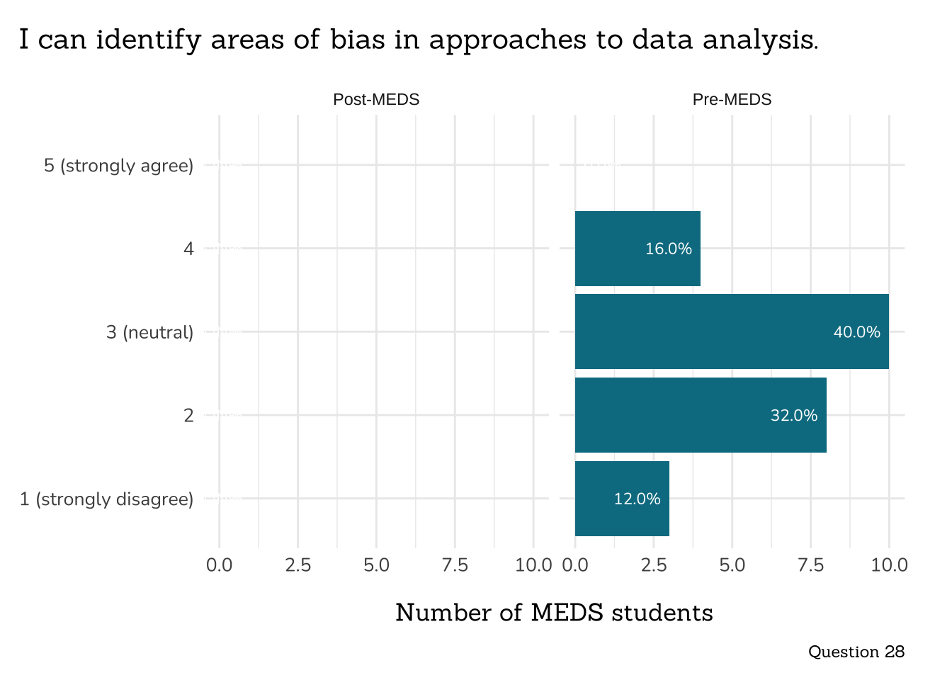plot_rank_data(data = q28_bias_data, title = "I can identify areas of bias in approaches to data analysis.", caption = "Question 28") ``` ## **Part 11: Data Viz & Communication** ```{r} ##~~~~~~~~~~~~~~~~~~~~~~~~~~~~~~~~~~~~~~ ## ~ Question 29: Create Data Viz ---- ##~~~~~~~~~~~~~~~~~~~~~~~~~~~~~~~~~~~~~~ # wrangle ---- q29_create_viz_data <- clean_freq_rank_data(all_PLO_data = meds2026_before_clean, #both_timepoints_clean, col_name = "data_viz_programming", categories = c("1 (never done it)", "2", "3", "4", "5 (very comfortable, do it often)")) # plot ---- 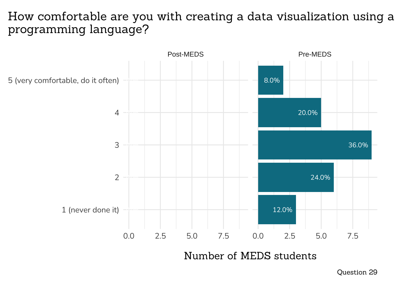plot_rank_data(data = q29_create_viz_data, title = "How comfortable are you with creating a data visualization using a\nprogramming language?", caption = "Question 29") ``` #### 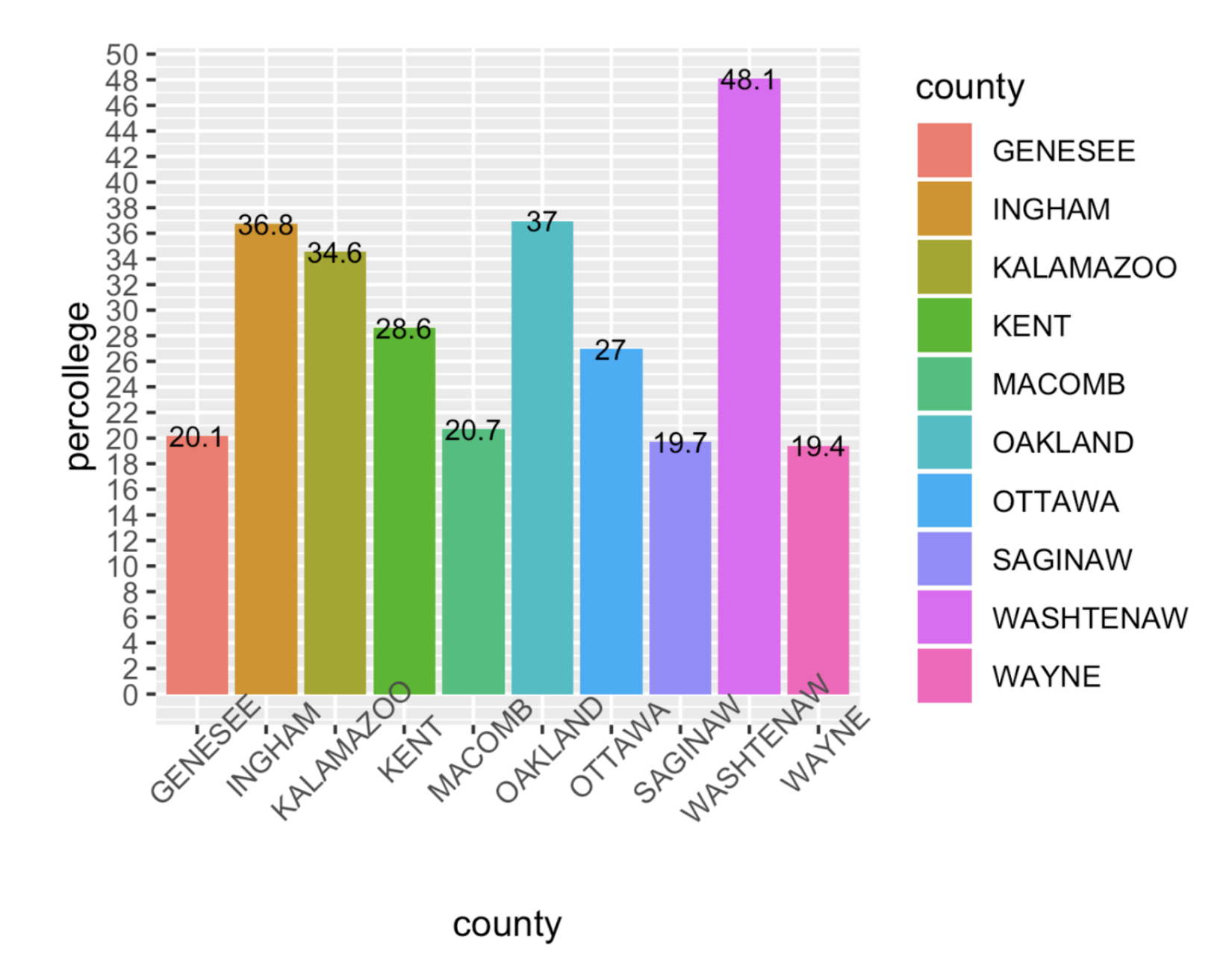Identify 4 areas for improvement in the following data visualization that shows information about Michigan counties with highest college attendance (Question 30). ```{r} #| fig-align: center knitr::include_graphics(here::here("yearly-reports", "images", "30-plot.png")) ``` ::: {.center-text .body-text-m} *Wordcloud of most frequently occurring words used to describe suggested improvements to the above data visualization (Question 30)* ::: :::: {.columns} ::: {.column width="50%"} ::: {.center-text} **Pre-MEDS** ::: ```{r} #| eval: true #| echo: false ##~~~~~~~~~~~~~~~~~~~~~~~~~~~~~~~~~~~~~~~~~~~~~~~~~~~~~~~~~~~~~~~~~~~~~~~~~~~~~~ ## Question 30: Improve Data Viz (Pre-MEDS) ---- ##~~~~~~~~~~~~~~~~~~~~~~~~~~~~~~~~~~~~~~~~~~~~~~~~~~~~~~~~~~~~~~~~~~~~~~~~~~~~~~ # wrangle ---- q30_improve_dv_pre <- clean_q30_improve_dv(meds2026_before_clean) # plot ---- plot_q30_improve_dv(q30_improve_dv_pre) ``` ::: ::: {.column width="50%"} ::: {.center-text} **Post-MEDS** ::: ```{r} # # ##~~~~~~~~~~~~~~~~~~~~~~~~~~~~~~~~~~~~~~~~~~~~~~~~~~~~~~~~~~~~~~~~~~~~~~~~~~~~~~ # ## Question 30: Improve Data Viz (Post-MEDS) ---- # ##~~~~~~~~~~~~~~~~~~~~~~~~~~~~~~~~~~~~~~~~~~~~~~~~~~~~~~~~~~~~~~~~~~~~~~~~~~~~~~ # # # wrangle ---- # q30_improve_dv_post <- clean_q30_improve_dv(meds2026_after_clean) # # # plot ---- # plot_q30_improve_dv(q30_improve_dv_post) ``` ::: :::: ::: {.callout-note collapse=true} ## Question 30 raw responses Responses as they were recorded are included in the tables, below: ```{r} #~..........................wrangle............................. q30_improve_dv_pre <- meds2026_before_clean |> #both_timepoints_clean |> # select necessary cols & arrange ---- select(timepoint, improve_data_viz) |> arrange(timepoint) #........................create DT table......................... DT::datatable(q30_improve_dv_pre, colnames = c("Timepoint", "Free Response Answer to Q30"), #caption = htmltools::tags$caption( style = 'caption-side: top; text-align: center; color:black; font-size:200% ;','Pre-MEDS:'), options = list(autoWidth = TRUE, pageLength = 5, lengthMenu = c(5, 10, 20, 30), dom = 'ltp') ) ``` ```{r} # ##~~~~~~~~~~~~~~~~~~~~~~~~~~~~~~~~~~~~~~~~~~~~~~~~~~~~~~~~~~~~~~~~~~~~~~~~~~~~~~ # ## Pre-MEDS ---- # ##~~~~~~~~~~~~~~~~~~~~~~~~~~~~~~~~~~~~~~~~~~~~~~~~~~~~~~~~~~~~~~~~~~~~~~~~~~~~~~ # # #~..........................wrangle............................. # q30_improve_dv_pre <- meds2026_before_clean |> # # # select necessary cols ---- # select(improve_data_viz) # # #........................create DT table......................... # DT::datatable(q30_improve_dv_pre, colnames = c("Free Response Answer to Q30"), # # caption = htmltools::tags$caption( style = 'caption-side: top; text-align: center; color:black; font-size:200% ;','Pre-MEDS:'), # # options = list(autoWidth = TRUE, # pageLength = 5, # lengthMenu = c(5, 10, 20, 30), # dom = 'ltp') # # ) ``` ```{r} #| eval: false # ##~~~~~~~~~~~~~~~~~~~~~~~~~~~~~~~~~~~~~~~~~~~~~~~~~~~~~~~~~~~~~~~~~~~~~~~~~~~~~~ # ## Post-MEDS ---- # ##~~~~~~~~~~~~~~~~~~~~~~~~~~~~~~~~~~~~~~~~~~~~~~~~~~~~~~~~~~~~~~~~~~~~~~~~~~~~~~ # # #~..........................wrangle............................. # q30_improve_dv_post <- meds2026_after_clean |> # # # select necessary cols ---- # select(improve_data_viz) # # #........................create DT table......................... # DT::datatable(q30_improve_dv_post, colnames = c("Free Response Answer to Q30"), # # caption = htmltools::tags$caption( style = 'caption-side: top; text-align: center; color:black; font-size:200% ;','Prost-MEDS:'), # # options = list(autoWidth = TRUE, # pageLength = 5, # lengthMenu = c(5, 10, 20, 30), # dom = 'ltp') # # ) ``` ::: ## **Part 12: Programming 2** ```{r} #| eval: false #| echo: true # define function 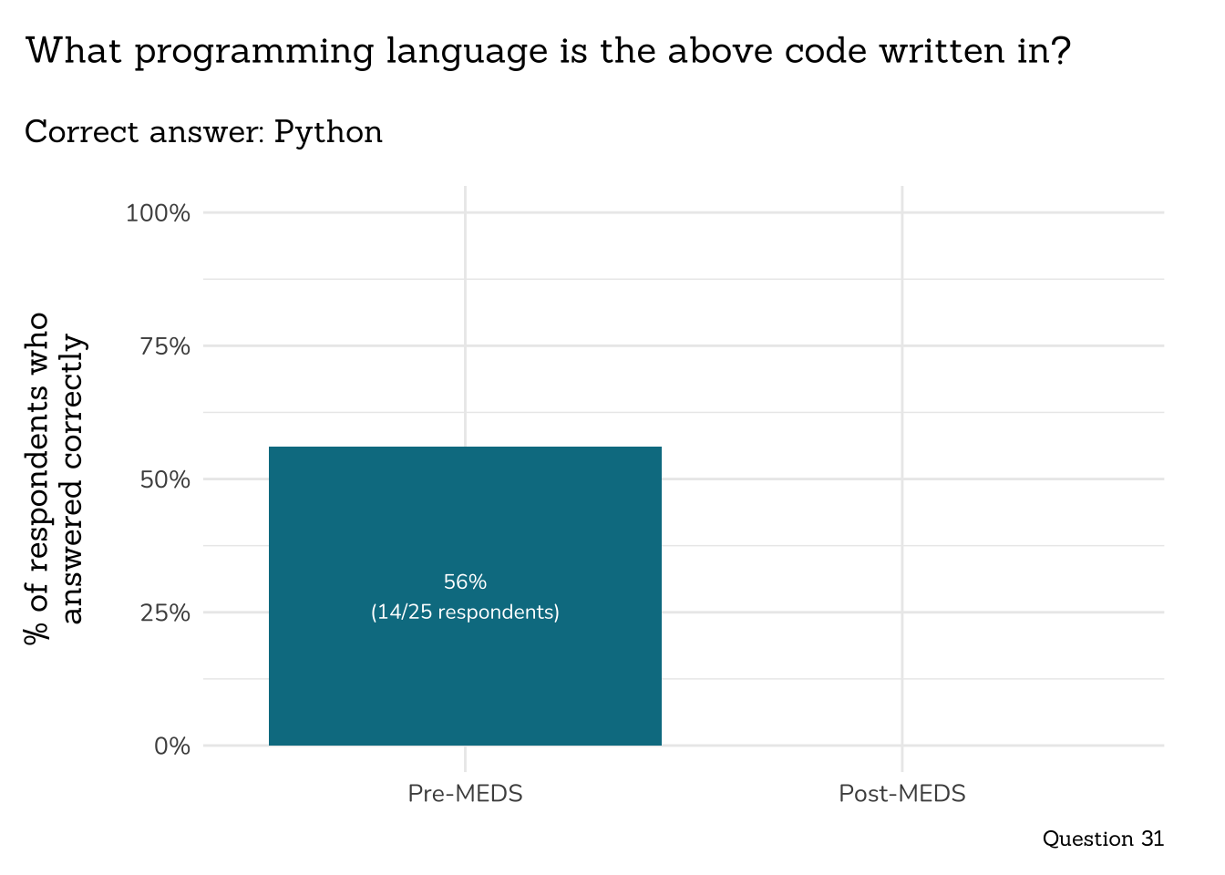def convert_F_to_C(temp_F): temp_C = (temp_F-32)*5/9 return temp_C # use function convert_F_to_C(32) ``` ```{r} ##~~~~~~~~~~~~~~~~~~~~~~~~~~~~~~~~~~~~ ## ~ Question 31: What Language ---- ##~~~~~~~~~~~~~~~~~~~~~~~~~~~~~~~~~~~~ # wrangle ---- q31_lang_data <- clean_q31_lang(meds2026_before_clean) # both_timepoints_clean # plot ---- plot_correct_answer_comparison(data = q31_lang_data, title = "What programming language is the above code written in?", subtitle = "Correct answer: Python", caption = "Question 31") ``` <br> ::: {.center-text} ***End MEDS Class of 2026 PLO Assessment Report*** ::: <br> ::: {.center-text} *Return to [main page](../index.html)* :::